Learning Objectives

• Review cokriging.
• Understand the development of the Markov Models.
• Demonstrate (intrinsic) collocated cokriging with Markov model II
• Understand a workflow for collocated cokriging (source code available).

Introduction

Consider two coregionalized variables \(Z(\textbf{u})\), the primary variable, and \(Y(\textbf{u})\), the secondary variable where \(\textbf{u}\) refers to locations in a stationary domain. The primary variable \(Z(\textbf{u})\) is sampled at \(n\) locations. The secondary variable \(Y(\textbf{u})\) is measured at all locations within the domain. The \(Y(\textbf{u})\) variable is used to inform the prediction of \(Z(\textbf{u})\). Only one secondary variable is considered for this lesson; if multiple secondary variables are present, the simplest solution is to aggregate secondary variables into one super secondary variable (see the lesson on supersecondaries). The complete implementation is demonstrated in an accompanying Python notebook.

Cokriging uses the resulting aggregated super secondary variable (Yang & Deutsch (2019)). Traditionally cokriging with a linear model of coregionalization (LMC) is used in multivariate estimation; however, due to the complexity of the cokriging workflow, other techniques were developed for scenarios with exhaustively sampled secondary data. Collocated cokriging simplifies estimation by using an intrinsic model and the collocated secondary data. This lesson will explain and compare the different methods of collocated cokriging. To help simplify the lesson it will be assumed that the variables \(Z(\textbf{u})\) and \(Y(\textbf{u})\) have been standardized or normal score transformed and have a mean of zero and a standard deviation of one (see the lesson on the normal score transformation).

Correlogram Review

The spatial variability of the primary, secondary, and between the primary and secondary variables must be considered. The spatial variablity is described by the variogram or correlogram (see the lesson on the pairwise relative variogram). It is assumed that the variables are stationary. The correlogram for \(Z(\textbf{u})\) can be defined as:

\[ {\rho_z}(\mathbf{h}) = E\left [ Z(\mathbf{u})Z(\mathbf{u}+\mathbf{h})) \right ] \]

where \(\mathbf{h}\) is a lag vector, similarly the correlogram for \(Y(\textbf{u})\) can be defined as:

\[ {\rho_y}(\mathbf{h}) = E\left [ Y(\mathbf{u})Y(\mathbf{u}+\mathbf{h})) \right ] \]

The cross-correlogram can be defined as:

\[ \rho_{zy}(\textbf{h}) = E\left [ Z(\mathbf{u})Y(\mathbf{u}+\mathbf{h})) \right ] \]

For example, the cross-correlogram can be estimated in this fashion:

\[ \hat{\rho_{zy}}(\textbf{h}) = \frac{1}{N(\textbf{h})} \sum_{i=1}^{N(\textbf{h})} Z(\mathbf{u_i}) Y(\mathbf{u_i+h}) \]

where \(N(\textbf{h})\) pairs of samples are separated by the lag vector \(\textbf{h}\) (note that bold variables represent a set of values). The direct \(Z\) and \(Y\) correlograms are estimated in a similar fashion. Note that the correlogram can capture the lag effect,that is, \(\rho_{zy}(\textbf{h})\neq\rho_{yz}(\textbf{h})\).

A linear model of coregionalization could be used to model spatial continuity of the variables. The LMC is modeled with the same pool of nested structures and must be modeled to ensure that the resulting kriging matrix is positive definite. The LMC can be denoted as:

\[ \rho_{z}(\mathbf{h}) = 1 - \sum_{k=0}^{nst}b^{k}_{z}C^{k}(\mathbf{h}) \\ \rho_{y}(\mathbf{h}) = 1 - \sum_{k=0}^{nst}b^{k}_{y}C^{k}(\mathbf{h}) \\ \rho_{yz}(\mathbf{h}) = \sum_{k=0}^{nst}b^{k}_{yz}C^{k}(\mathbf{h}) \]

Where:

• \(C^{k}(\mathbf{h})\) are the pool of \(k = 0,...,nst\) structures, where the \(0^{th}\) nested structure is the nugget effect by convention
• \(b^k\) is the contribution of each structure

In a LMC the \(b^k\) coefficients may vary, but they are constrained to yield a positive definite model:

\[ b^k_z \times b^k_{y} \geq (b^k_{yz})^2 \hspace{1.0em} k = 0,...,nst \]

More on LMC’s can be found in Goulard & Voltz (1992).

Simple Cokriging Review

Simple Cokriging (SCK) is an extension of kriging for modeling multivariate problems. SCK considers the primary and secondary data available. SCK does not require equal sampling of the primary and secondary data which is an advantage over many other multivariate techniques. The equations for SCK:

\[ Z^{*}(\mathbf{u_{0}}) = \sum_{\alpha=1}^{n}\lambda_{Z,\alpha}Z(\mathbf{u}_{\alpha})+ \sum_{\alpha=1}^{n_y}\lambda_{Y,\alpha}Y(\mathbf{u}_{\alpha}) \]

The system of equations to solve for the SCK weights:

\[ \left\{\begin{matrix} \hspace{-0.75em}\sum_{\alpha=1}^{n}\lambda_{Z,\alpha}\rho_{z}(\mathbf{u}_\alpha-\mathbf{u_{\beta}})+ \sum_{\alpha=1}^{n_y}\lambda_{Y_{\alpha}} \rho_{yz}(\mathbf{u}_\alpha-\mathbf{u}_\beta) = \rho_{z}(\mathbf{u}_\beta-\mathbf{u}_0)\\ \beta = 1,...,n\\ \sum_{\alpha=1}^{n_y}\lambda_{Z,\alpha}\rho_{yz}(\mathbf{u}_\alpha-\mathbf{u_{\beta}})+ \sum_{\alpha=1}^{n}\lambda_{Y_{\alpha}} \rho_{y}(\mathbf{u}_\alpha-\mathbf{u}_\beta) = \rho_{yz}(\mathbf{u}_\beta-\mathbf{u}_0)\\ \beta = 1,...,n_y\\ \end{matrix}\right. \]

Where:

• \(\rho_{z}(\mathbf{u}_\alpha-\mathbf{u}_{\beta}), \alpha,\beta =1,...n\) are the spatial correlations between primary data calculated based on the \(\rho_{z}(\mathbf{h})\) correlogram
• \(\rho_{yz}(\mathbf{u}_\alpha-\mathbf{u}_{0})\) and \(\rho_{yz}(\mathbf{u}_\alpha-\mathbf{u}_\beta) \alpha,\beta =1,...n\) are the spatial cross-correlations between primary and secondary data calculated based on the \(\rho_{yz}(\mathbf{h})\) cross correlogram
• \(\rho_{y}(\mathbf{u}_\alpha-\mathbf{u}_\beta)\) is the spatial correlation between the secondary data calculated based on the \(\rho_{y}(\mathbf{h})\) correlogram
• \(\lambda_{Z,\alpha}\) is the kriging weight for the \(\alpha^{th}\) primary data sample for \(\alpha = 1,...n\)
• \(\lambda_{Y,\alpha}\) is the kriging weight for the \(\alpha^{th}\) secondary data sample for \(\alpha = 1,...n_y\)

Cokriging is very useful; however, calculating, interpreting, and fitting the correlograms required for an LMC could be tedious. If the secondary data are exhaustively sampled, we are motivated to simplify the estimation (Rossi & Deutsch (2014)).

The Markov Models

Collocated cokriging and the Markov model I (MMI) were introduced as a simpler method of modeling multivariate geological problems in the presence of exhaustive secondary data (Almeida & Journel (1994)). The MMI uses the primary correlogram and the correlation between the primary and secondary data to infer all correlations. The Markov model II (MMII) is a similar method; however, uses the correlogram of the secondary variable, a residual correlogram, and the correlations between the secondary and primary data are needed to calculate all correlations.

Markov Model I

The Markov Model cross-correlogram is expressed as:

\[ \rho_{yz}(\boldsymbol{h}) = \rho_{yz}(0)\rho_{z}(\boldsymbol{h}) \]

Where \(\rho_{z}(\boldsymbol{h})\) is the primary variable correlogram and \(\rho_{yz}(\boldsymbol{h})\) is the cross-correlogram between the primary variable \(Z(\boldsymbol{h})\) and the secondary variable \(Y(\boldsymbol{h})\). \(\rho_{yz}(0)\) is the collocated correlation coefficient.

The MMI does not require the correlogram of the secondary variable it is assumed that:

\[ \rho_{y}(\boldsymbol{h}) = \rho_{z}(\boldsymbol{h}) \]

The assumption is that \(\rho_{yz}(\boldsymbol{h})\) and \(\rho_{z}(\boldsymbol{h})\) have the same shape and continuity; however, the MMI can produce suboptimal results (Shmaryan & Journel (1999)).

Markov Model II

The Markov model II (MMII) was developed assuming that the secondary variable \(Y(\boldsymbol{h})\) is more stable then the primary variable \(Z(\boldsymbol{h})\). The cross-correlogram is related to the secondary correlogram:

\[ \rho_{yz}(\boldsymbol{h}) = \rho_{yz}(0)\rho_{y}(\boldsymbol{h}) \]

The primary correlogram \(\rho_{z}(\boldsymbol{h})\) is then calculated with the secondary correlogram \(\rho_{y}(\boldsymbol{h})\):

\[ \rho_{z}(\boldsymbol{h}) = \rho_{yz}^2(0)\rho_{y}(\boldsymbol{h})+(1-\rho_{yz}^2(0))\rho_{r}(\boldsymbol{h}) \]

where \(\rho_{r}(\boldsymbol{h})\) is fit such that:

\[ \rho_{z}(\boldsymbol{h}) \approx \hat{\rho}_{z}(\boldsymbol{h}) \]

The key idea is that \(\rho_{yz}^2(0)\) is the minimum contribution of \(\rho_{y}\) to maintain positive definiteness. The major difference between MMI and MMII is that the cross-correlogram \(\rho_{yz}(\boldsymbol{h})\) in the MMI uses \(\rho_{z}(\boldsymbol{h})\) and the MMII uses \(\rho_{y}(\boldsymbol{h})\). Once the method of determining how to calculate the correlograms is established the next step is to determine the kriging method to implement.

Summary of the Markov Model Correlograms Calculations

A summary of the Markov Models is shown below.

\[ \begin{matrix} \mathrm{Correlogram}&\mathrm{Markov\,Model 1}&\mathrm{Markov\,Model 2} \\ \hline \rho_{z}(\boldsymbol{h})= & \rho_{z}(\boldsymbol{h}) & \rho_{yz}^2(0)\rho_{y}(\boldsymbol{h})+(1-\rho_{yz}^2(0))\rho_{r}(\boldsymbol{h})\\ \rho_{yz}(\boldsymbol{h})=& \rho_{z}(\boldsymbol{h})\rho_{yz}(0)& \rho_{y}(\boldsymbol{h})\rho_{yz}(0)\\ \rho_{y}(\boldsymbol{h})= & \rho_{z}(\boldsymbol{h}) & \rho_{y}(\boldsymbol{h}) \end{matrix} \]

Kriging

Simple Collocated Cokriging

Simple collocated cokriging (SCCK) is widely accepted in the practices of geostatistics as an alternative to Cokriging with an LMC (Shmaryan & Journel (1999)). The equation for SCCK is:

\[ Z^{*}(\mathbf{u}_{0}) = \sum_{\alpha=1}^{N}\lambda_{\alpha}Z(\mathbf{u}_{\alpha})+ \lambda_{Y_0}Y(\mathbf{u}_{0}) \]

where \(Z^{*}(\mathbf{u}_0)\) is the estimate at the unsampled location, \(Y(\mathbf{u}_{0})\) is the value secondary variable at the estimation location and the \(\lambda\)’s are the kriging weights. The kriging weights are solved from the following system of equations using MMI or MMII:

\[ \left\{\begin{matrix} \sum_{\alpha=1}^{n}\lambda_{Z,\alpha}\rho_{z}(\mathbf{u}_\alpha-\mathbf{u_{\beta}})+ \lambda_{Y_{0}}\rho_{yz}(\mathbf{u}_\beta-\mathbf{u}_0) = \rho_{z}(\mathbf{u}_\beta-\mathbf{u}_0),\beta = 1,...,n\\ \hspace{-13.5em}\sum_{\alpha=1}^{n}\lambda_{Z,\alpha}\rho_{yz}(\mathbf{u}_\alpha-\mathbf{u_{0}})+ \lambda_{Y_{0}} = \rho_{yz}(0)\\ \end{matrix}\right. \]

Where:

• \(\rho_{z}(\mathbf{u}_\alpha-\mathbf{u}_{\beta}), \alpha,\beta =1,...n\) are the spatial correlation between primary data calculated with the \(\rho_{z}(\mathbf{h})\) correlogram
• \(\rho_{yz}(\mathbf{u}_\alpha-\mathbf{u}_{0}), \beta =1,...n\) are the spatial cross-correlation between primary and secondary data calculated with the \(\rho_{yz}(\mathbf{h})\) correlogram
• \(\lambda_\alpha\) is the kriging weight for the \(\alpha^{th}\) primary data sample for \(\alpha = 1,...n\)
• \(\lambda_{Y_0}\) is the kriging weight for the secondary collocated data

Although simple collocated cokriging is a more straightforward workflow compared to cokriging, there is a drawback. Simple cokriging results in variance inflation in the estimation, and the estimate is less accurate than cokriging. The variance inflation is due to the collocated system of equations not being an exact intrinsic model (Babak & Deutsch (2007)). Using a true intrinsic model corrects variance inflation and improves the results.

Intrinsic Collocated Cokriging

ICCK includes all secondary data from the primary locations and the collocated location; the variance is more accurately reproduced and variance inflation does not occur (Babak & Deutsch (2007)). The ICCK estimate is written:

\[ Z^{*}(\mathbf{u_{0}}) = \sum_{\alpha=1}^{n}\lambda_{Z,\alpha}Z(\mathbf{u}_{\alpha})+ \sum_{\alpha=1}^{n}\lambda_{Y,\alpha}Y(\mathbf{u}_{\alpha})+ \lambda_{Y,0}Y(\mathbf{u}_{0}) \]

The system of equations to solve for the ICCK weights is:

\[ \left\{\begin{matrix} \hspace{-0.5em}\sum_{\alpha=1}^{n}\lambda_{Z,\alpha}\rho_{z}(\mathbf{u}_\alpha-\mathbf{u_{\beta}})+ \sum_{\alpha=1}^{n}\lambda_{Y_{\alpha}} \rho_{yz}(\mathbf{u}_\alpha-\mathbf{u}_\beta)+ \lambda_{Y_{0}}\rho_{yz}(\mathbf{u}_\beta-\mathbf{u}_0) = \rho_{z}(\mathbf{u}_\beta-\mathbf{u}_0)\\ \beta = 1,...,n\\ \sum_{\alpha=1}^{n}\lambda_{Z,\alpha}\rho_{yz}(\mathbf{u}_\alpha-\mathbf{u_{\beta}})+ \sum_{\alpha=1}^{n}\lambda_{Y_{\alpha}} \rho_{y}(\mathbf{u}_\alpha-\mathbf{u}_\beta)+ \lambda_{Y_{0}}\rho_{y}(\mathbf{u}_\beta-\mathbf{u}_0) = \rho_{yz}(\mathbf{u}_\beta-\mathbf{u}_0)\\ \beta = 1,...,n\\ \hspace{-7.75em}\sum_{\alpha=1}^{n}\lambda_{Z,\alpha}\rho_{yz}(\mathbf{u}_\alpha-\mathbf{u_{0}})+ \sum_{\alpha=1}^{n}\lambda_{Y_{\alpha}} \rho_{y}(\mathbf{u}_\alpha-\mathbf{u}_0)+ \lambda_{Y_{0}} = \rho_{yz}(0)\\ \end{matrix}\right. \]

Where:

• \(\rho_{z}(\mathbf{u}_\alpha-\mathbf{u}_{\beta}), \alpha,\beta =1,...n\) are the spatial correlation between primary data calculated with the \(\rho_{z}(\mathbf{h})\) correlogram
• \(\rho_{yz}(\mathbf{u}_\alpha-\mathbf{u}_{0})\) and \(\rho_{yz}(\mathbf{u}_\alpha-\mathbf{u}_\beta), \alpha,\beta =1,...n\) are the spatial cross-correlation between primary and secondary data
• \(\lambda_{Z,\alpha}\) is the kriging weight for the \(\alpha^{th}\) primary data sample for \(\alpha = 1,...n\)
• \(\lambda_{Y,\alpha}\) is the kriging weight for the \(\alpha^{th}\) secondary data sample for \(\alpha = 1,...n\)
• \(\lambda_{Y_0}\) is the kriging weight for secondary collocated data

Although ICCK solves the variance inflation issues, it requires almost double the size of the matrix for solving the kriging weights; however, with today’s computational power, this is not a significant problem.

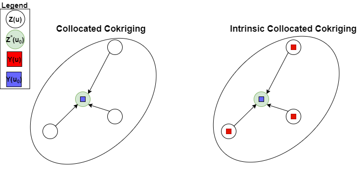
The figure below illustrates the difference between SCCK and ICCK. In SCCK(left) only the primary data(\(Z(\mathbf{u})\)), represented by open circles, and the collocated data(\(Y(u_0)\)), represented by a blue square, are used to calculate the estimate(\(Z^*(u_0)\)), represent by a tan circle. In ICCK(right), the primary data, the collocated data, and the secondary data at all primary data locations (\(Y(\mathbf{u})\)), represented by red squares, are used to make the estimate. The arrow in the diagrams would represent the correlogram lag distance used to calculate the spatial correlation.

Example

To illustrate the four different methods of making an estimate using SCCK and ICCK with MMI/MMII a 2D example is explored below (with source code in accompanying notebook).

Data

The figure below shows the primary data \(Z(\mathbf{u})\) on the left and the exhaustive secondary data \(Y(\mathbf{u})\) on the right.

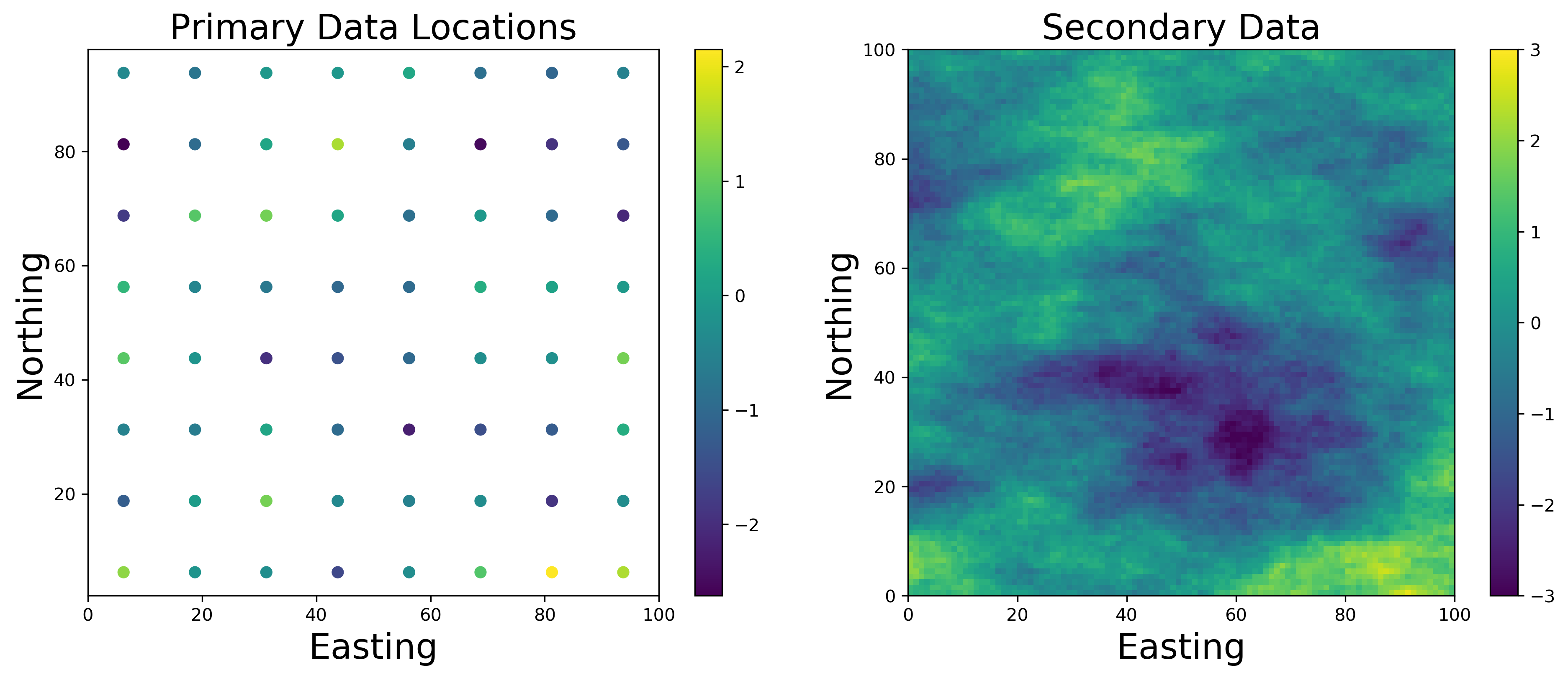
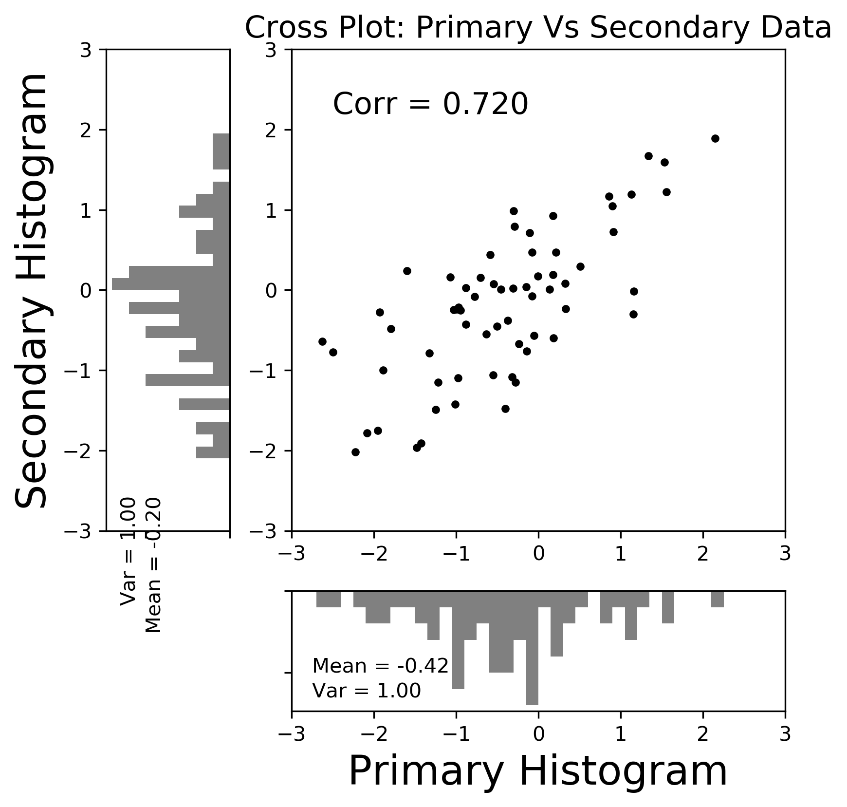
From the histograms and scatter plot below the data has a reasonably strong correlation, \(\rho_{yz(0)}\), of \(0.72\). The mean and variance of the primary data is \(-0.42\) and \(1.00\) respectively.The mean and variance of the secondary data is \(0.20\) and \(1.00\), respectively. The data was sampled from a Gaussian simulation.

The next step is to model the correlogram of both the primary and secondary data. From the exhaustive data map the major direction of continuity appears to be \(90^{\circ}\). In MMI the primary correlogram \(\rho_{z_{Model}}(\boldsymbol{h})\) and the correlation is used to calculate the correlations in the Kriging equations. In MMII the secondary correlogram \(\rho_{y_{Model}}(\boldsymbol{h})\) and the correlation is used to calculate the secondary covariance and the cross covariance. In MMII the primary covariance is fit using \(\rho_{r}(\boldsymbol{h})\) and the secondary correlogram \(\rho_{y_{Model}}(\boldsymbol{h})\). The primary correlogram for the MMII is denoted as \(\rho_{z_{MMII}}(\boldsymbol{h})\) in the images below. \(\rho_{z_{MMII}}(\boldsymbol{h})\) should be similar to \(\rho_{z_{Model}}(\boldsymbol{h})\).

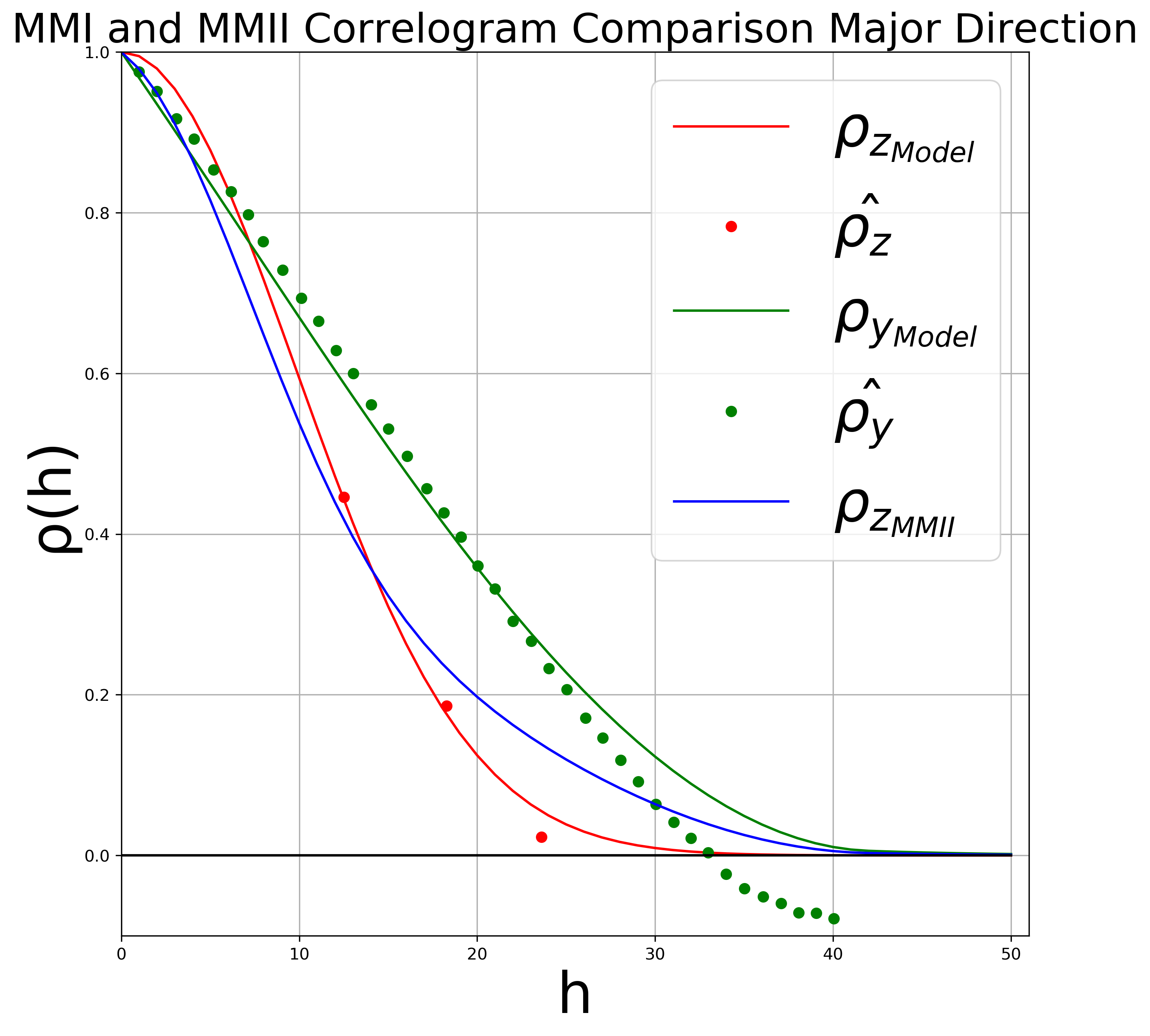
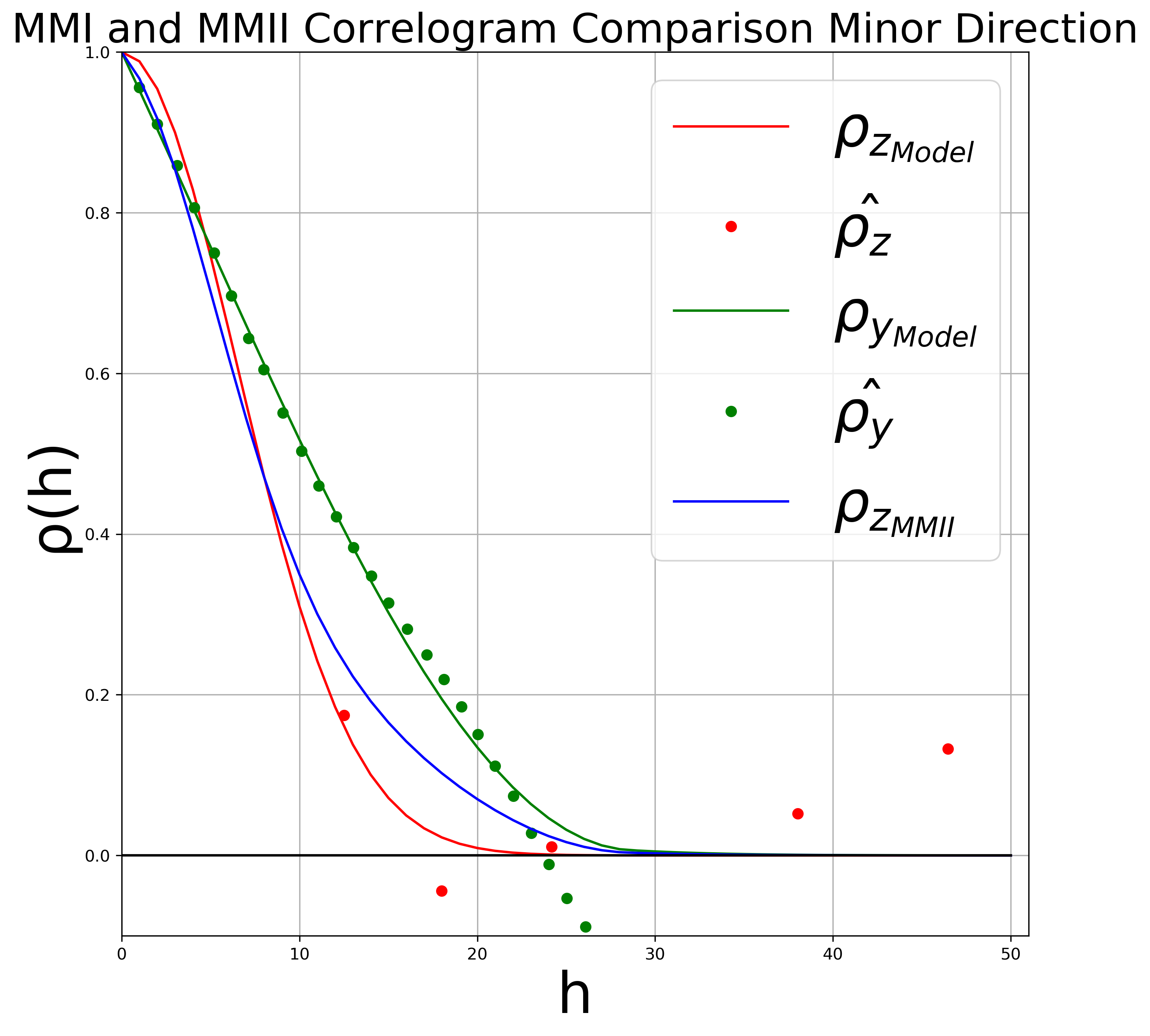
The correlograms can be written as:

\[ \rho_{z_{Model}}(\boldsymbol{h}) = 1.00 Gaussian_{\begin{matrix} a1_{maj} = 24 \\ a1_{min} = 16 \end{matrix}} \]

\[ \rho_{y_{Model}}(\boldsymbol{h}) = 0.9 Spherical_{\begin{matrix} a1_{maj} = 42\\ a1_{min} = 28.5 \end{matrix}} +0.1 Gaussian_{\begin{matrix} a2_{maj} = 43 \\ a2_{min} = 30 \end{matrix}} \]

Where the primary correlogram has one Gaussian structure with a range of 24 units in the major direction (\(a1_{maj}\)) and a range of 16 units in the minor direction (\(a1_{min}\)). The secondary correlogram modeled has two structures; the first structure, Spherical, contributes \(90\%\) of the correlogram with a major range of 42 units (\(a1_{maj}\)) and a minor range of 28.5 units (\(a1_{min}\)). The second structure, Gaussian, contributes the remaining \(10\%\) of the correlogram with a major range continuing to 42 units (\(a2_{maj}\)) and minor range continuing to 30 units (\(a1_{min}\)). More on variogram/correlogram structures can be found in Deutsch (2003).

Kriging

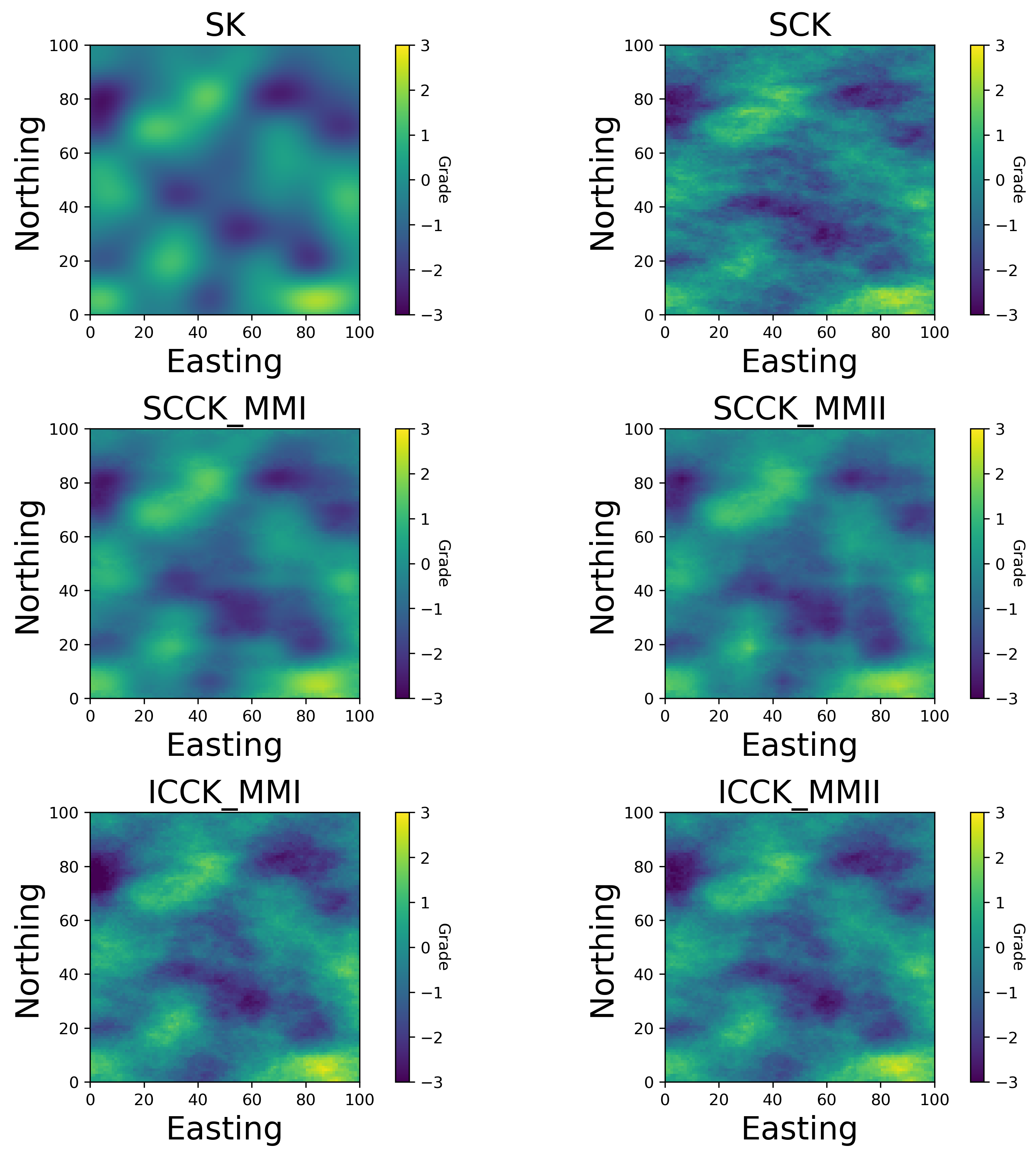
Kriging is performed with the 60 nearest data. The results from all four Kriging methods and SK/SCK(as a reference) are below. As expected, all methods produce very similar results; however, the MMII appears less smooth and more similar to SCK then the MMI.

Modeling Checking

A reference truth, \(Z^{True}(\mathbf{u})\), to this example is known, making it straightforward to compare each estimation method. Comparing each estimate root mean squared error (RMSE) illustrates the relative performance. The RMSE measures the difference between the true values and the predicted values:

\[ RMSE = \sqrt{ \frac{\sum_{i=0}^{n_{samples}}(Z^{True}(\mathbf{u_i})-Z^*(\mathbf{u_i}))^2} {n_{samples}}} \]

The error between the estimate and truth is shown below. As expected SK performs the worst and SCK performs the best; however, the ICCK MMII performs very similarly to SCK due to the MMII correlograms being close to the LMC correlograms.

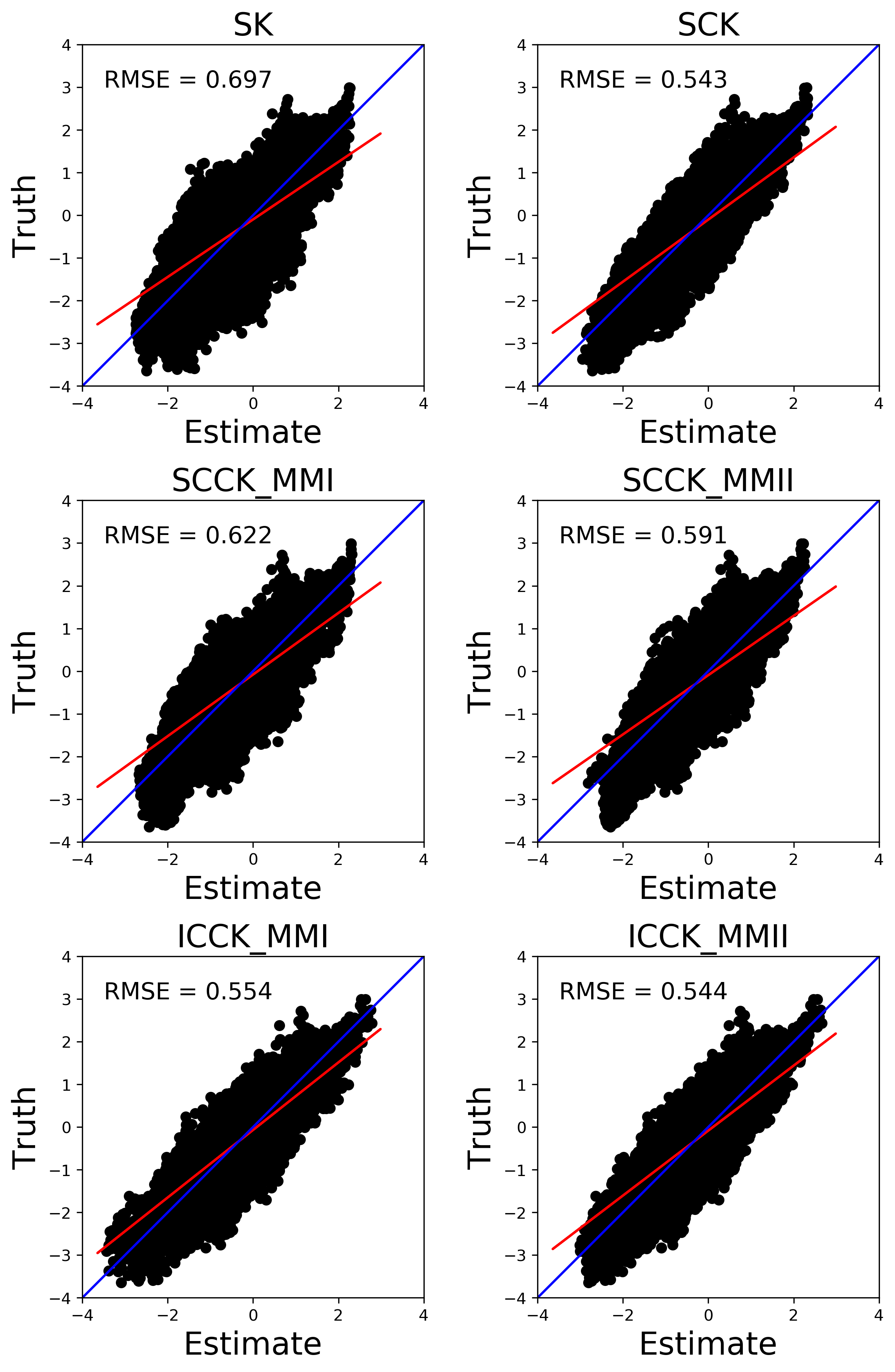
All methods are unbiased, smooth, and reproduce the distribution of the data reasonably well.

For the example demonstrated above using the MMII with ICCK would be recommended. Using MMII with ICCK results in almost the same results as SCK without the difficulties involved with fitting a valid LMC. For this example, the data was simulated using the MMII correlograms; hence, fitting the MMII correlograms was straight forward and results in a similar estimate to SCK. In practice, the MMII correlograms and LMC might not always be the same. ICCK with MMI is widely used in practice.

Conclusion

The Markov model I was developed as a simpler method for multivariate spatial estimation. The MMI uses the primary correlogram and the correlation between the primary and secondary data to calculate the cross-correlogram. It is assumed that the secondary correlogram is equal to the primary correlogram.

The Markov model II is used when the primary correlogram is not stable, or the primary data is sparsely sampled. The MMII uses the secondary correlogram and the correlations between the primary and secondary data to calculate the cross-correlogram. The primary correlogram is a combination of the secondary correlogram and a residual correlogram for fitting.

Simple Collocated Cokriging is not a true intrinsic model leading to variance inflation in estimation. Intrinsic Collocated Cokriging is used to eliminate the variance inflation by including all the secondary data at the primary data locations used for the estimate, not just the secondary data at the estimation location. Both MMI and MMII require exhaustive secondary data. For the example shown here, all four estimation techniques result in reasonable estimations with the ICCK MMII performing the best. Bayesian updating is another multivariate estimation technique that would produce similar results to collocated simple kriging. More on Bayesian Updating can be found in the lesson on Bayesian Updating for Combining Conditional Distributions and lesson on Bayesian Mapping.

References