Learning Objectives

• Review Bayes Theorem with an application in geostatistics.
• Motivate Bayes Theorem for secondary data integration.
• Understand a workflow for geostatistical modeling with secondary data (source code available).

Introduction

Uncertainty exists in rock properties at unsampled locations because of geological variability at all scales and relatively sparse sampling. Predicting local uncertainty is straightforward when a multivariate probability distribution of the unsampled value and all data can be constructed. The required conditional distribution is extracted directly from the multivariate distribution. In practice, a slightly different problem exists, that is, the integration of different data sources in the probabilistic prediction. There are times when Bayes Theorem naturally lends itself to assist in the integration of disparate data types. This Lesson reviews Bayes Theorem and shows an application to spatial prediction in presence of secondary data.

Although Bayes Theorem is extensively taught in Statistics, many geoscientists have limited statistics coursework or the courses are taught too early in their degree program for the context of Bayes Theorem to be made clear. The concept of updating an initial or prior understanding to an updated or posterior probability sounds reasonable, but the details warrant further attention. This Lesson aims to provide some clarity to Bayes Theorem in spatial prediction. An application to a simple 2-D mapping problem is shown, with code and data available as a Python notebook.

Bayes Theorem

Following is a classic presentation and interpretation of Bayes Theorem. Consider \(A\) to be an event we are trying to predict. \(B\) is some evidence or data that informs on \(A\). The conditional probabilities of \(A|B\) and \(B|A\) are defined as:

\[ P(A|B) = \frac{ P(A \; \mbox{and} \; B) }{ P(B) } \;\;\; \mbox{and} \;\;\; P(B|A) = \frac{ P(A \; \mbox{and} \; B) }{ P(A) } \]

These relations are considered axiomatic and the direct arithmetic result of considering multivariate probabilities. They are combined into the familiar form of Bayes Theorem:

\[ P(A|B) = \frac{ P(B|A) P(A) }{ P(B) } \]

This could be rewritten into the following:

\[ P(A|B) = P(A) \cdot \frac{1}{P(B)} \cdot P(B|A) \]

• \(P(A|B)\) is the updated probability of \(A\) given \(B\) also called the posterior.
• \(P(A)\) is the initial estimate of the probability of \(A\) also called the prior.
• The combination of \(P(B|A)/P(B)\) is the degree that \(B\) supports \(A\).
• \(1/P(B)\) is the rarity of \(B\).
• \(P(B|A)\) is the relevance of \(B\) for predicting \(A\) also called the likelihood.

In many situations \(B\) is fixed and different \(A\)’s are being considered, then the posterior probabilities are written as proportional to the product of the prior and likelihood:

\[ P(A|B) \propto P(A) \cdot P(B|A) \]

There are many profound interpretations and calculations possible with this theorem. The focus here is the prediction of a regionalized variable \(A\) at locations \({\mathbf{u}}\) within a domain: \(\{ A({\mathbf{u}}), {\mathbf{u}} \in \mbox{Domain} \}\). Perhaps the best way to understand Bayes Theorem in the context of geostatistics is with an example application.

Example

Consider two rock types. \(A\) is rock type 1 and not-\(A\) is rock type 0. Thus, \(A({\mathbf{u}})\) is an indicator random variable at each location \({\mathbf{u}}\) in the domain of interest. Consider also a continuous secondary variable \(Y({\mathbf{u}})\) over the domain that provides some information on the rock type. Although the \(Y\) variable is measured at all locations it is considered in a probabilistic sense to inform on the \(A\) variable (probability of \(A\)) being predicted.

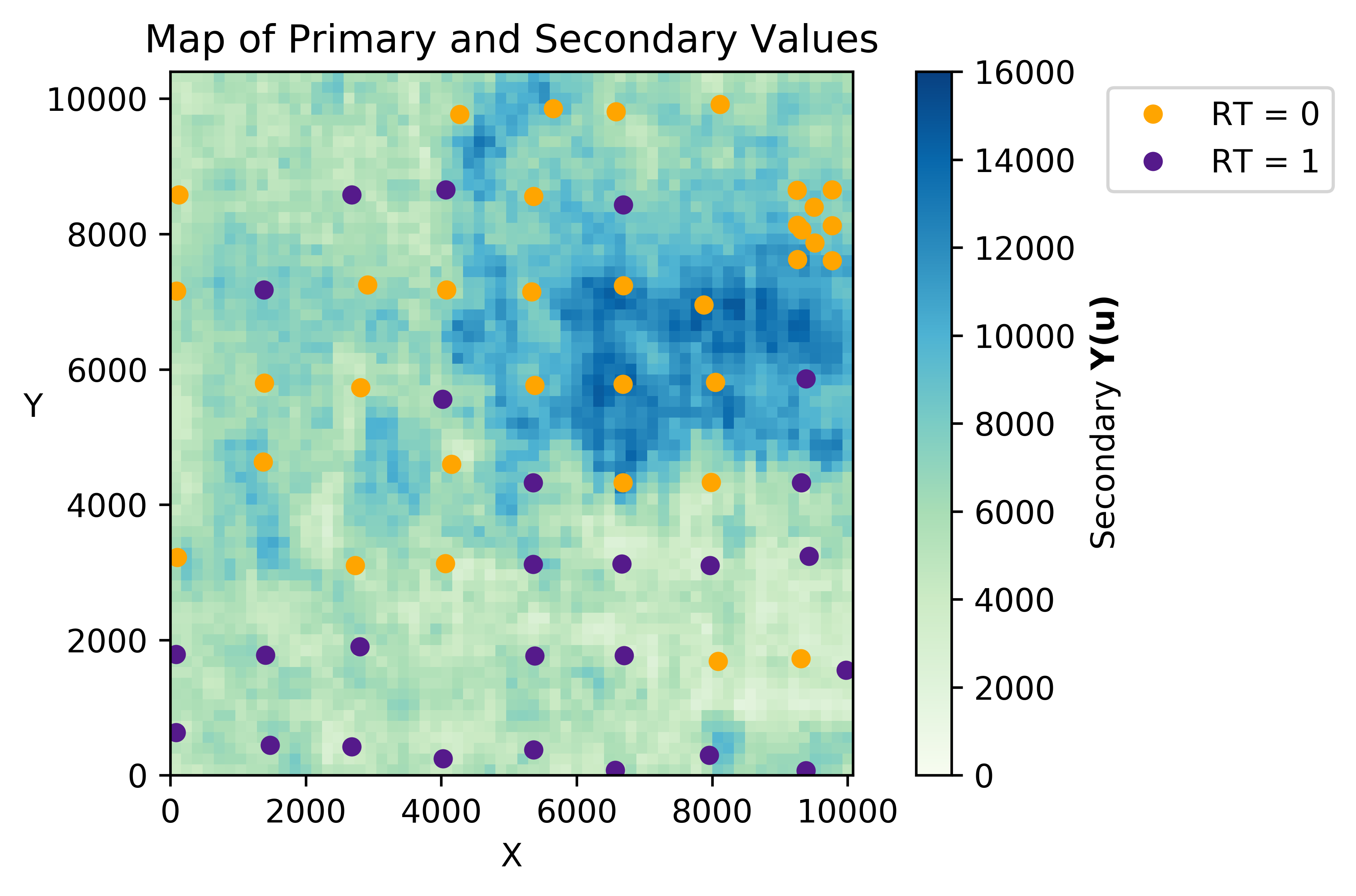
The goal is to predict \(P(A({\mathbf{u}})|y({\mathbf{u}}))\) that would be expressed as the following given the introduction to Bayes Theorem presented above:

\[ P(A({\mathbf{u}})|y({\mathbf{u}})) = P(A) \cdot \frac{1}{f_Y(y({\mathbf{u}}))} \cdot f_{Y|A}(y({\mathbf{u}})) \;\;\; {\mathbf{u}} \in \mbox{Domain} \]

This assumes a decision of stationarity for the initial \(P(A)\), knowledge of a deemed stationary marginal distribution of \(f_Y(y)\), and the likelihood distribution \(f_{Y|A}(y)\). The marginal distribution \(f_Y(y)\) is not strictly required since it does not depend on \(A\) or not-\(A\). The marginal stationary probabilities \(P(A)\) and \(P(\mbox{not}A)\) are calculated from the available data. A non-parametric estimate of these probabilities could be determined by the proportions of \(A\) and not-\(A\) in the data, but clustered data should be considered. Cell declustering (see the lesson on declustering) is considered and the declustered prior probabilities are determined to be \(P(A)=0.528\) and the complement \(P(\mbox{not}A)=0.472\).

Exhaustive data easily permits determination of \(f_Y(y)\). As mentioned, it is not needed since the conditional probabilities for \(A\) and not-\(A\) could be written as proportional to the prior and likelihood distribution without the marginal of \(Y\). Although not needed, the marginal distribution of \(Y\) is very well known because it is exhaustively measured and could be used to check future calculations.

Estimation of \(f_{Y|A}(y)\) and \(f_{Y|\mbox{not}A}(y)\) from the data may not be particularly reliable because of relatively few data. The histograms below show the distributions based on subsetting the \(Y\) values at locations of \(A\) and not-\(A\). These histograms have few data, so are moderately sensitive to the choice of binning.

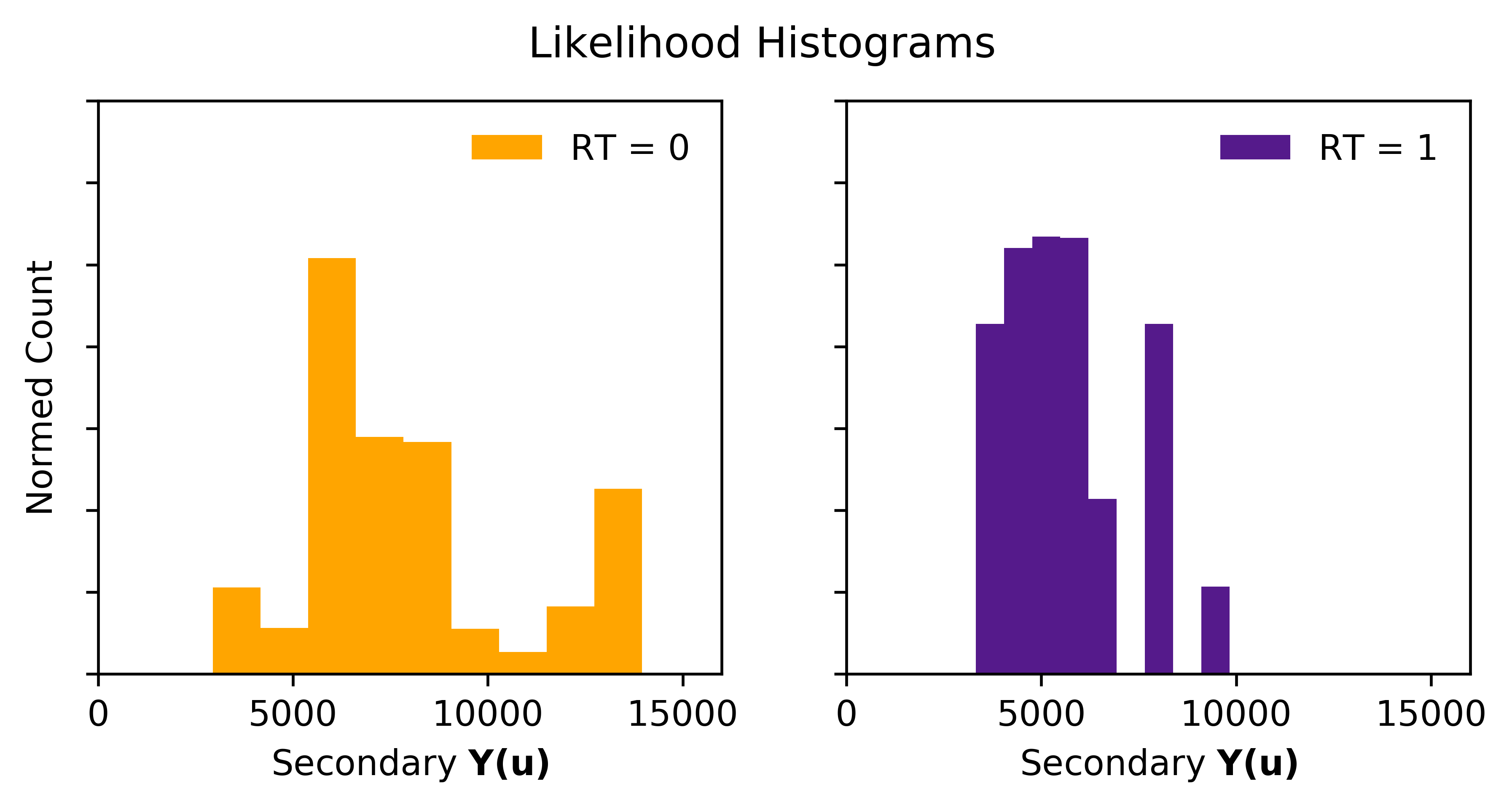
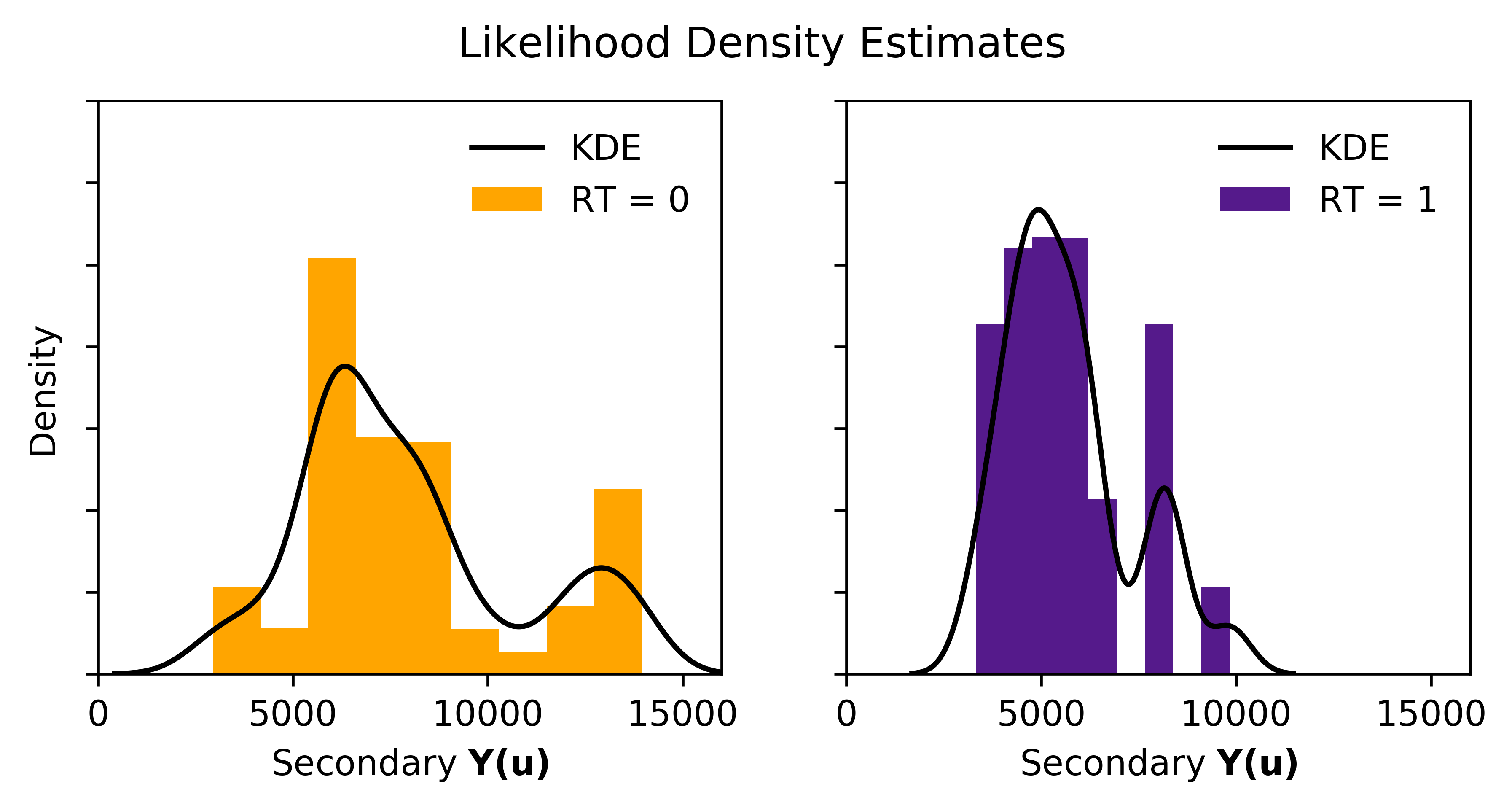
Although there are many secondary data the likelihood distributions must be inferred from the secondary data at the 61 locations where we know the primary variable of interest. Drilling or other direct observations of the primary variable is often expensive and there are few data. Fitting a parametric shape to the likelihood distributions is an attractive idea; however, most earth sciences data defy simple parameterization. Kernel density estimation (KDE) is a widely used non-parametric way to estimate the distribution of a random variable with few data. Each data is replaced by a kernel and an estimate of the distribution is the sum of the kernels. Consider a set of \(n\) data \((y_i,i=1,\ldots,n)\) and a kernel \(K\) that is non-negative and integrates to one. The estimated distribution is written as:

\[ \hat{f}_Y(y)=\frac{1}{n}\sum_{i=1}^n K_h(y-y_i) \]

where \(h\) is a smoothing parameter. There are many references on choosing the smoothing parameter, but Silverman’s rule of thumb is considered here (Silverman, 1986). A Gaussian kernel and optimal \(h\) parameter are given by:

\[ K_h(x)=\frac{1}{ h \sqrt{2 \pi}} e^{\frac{-x^2}{2h^2}} \;\;\; \mbox{and} \;\;\; h=\hat{\sigma} \frac{1.06}{n^{1/5}} \]

where \(\hat{\sigma}\) is the experimental standard deviation of the data. Note that the same declustering weights applied to the indicator \(A\) and not-\(A\) data would be applied to the \(Y\) data available at the data locations. Applying the kernel density estimator results in the following.

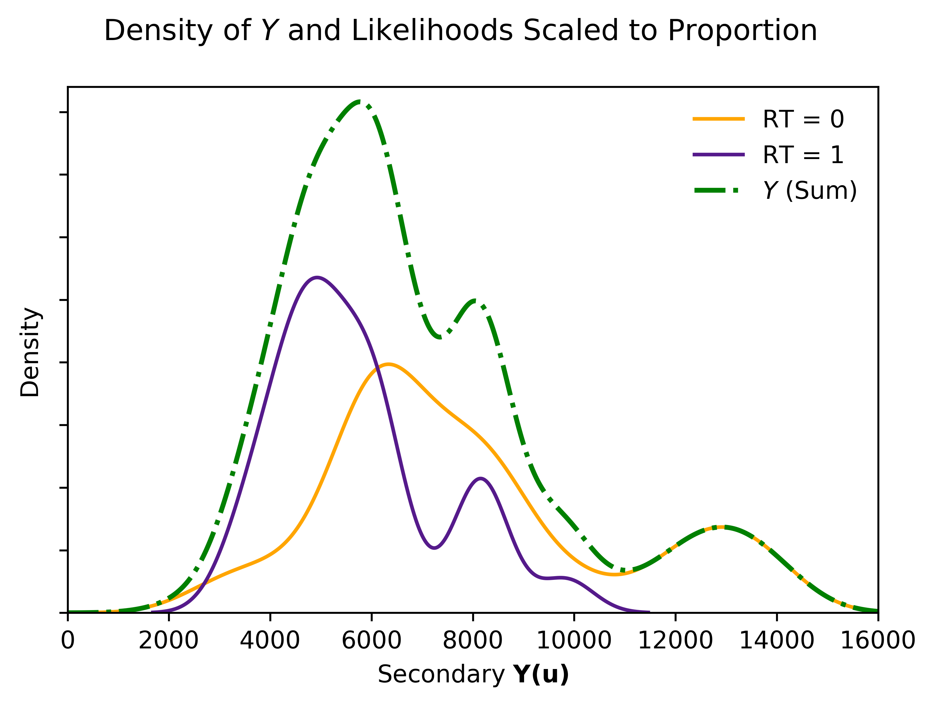
The weighted sum of these two marginal distributions should add up to the marginal of \(Y\) if the weighting is correct and the data are representative. In practice, they are rarely completely consistent. These likelihood distributions should be either restandardized to match the marginal \(f_Y(y)\) or the posterior probabilities restandardized if the “proportional to” interpretation is considered.

Calculating the posterior probabilities \(P(A({\mathbf{u}})|y({\mathbf{u}}))\) is straightforward with the prior probabilities and the likelihood distributions. The probability of \(\mbox{not}A\) is one minus this probability. The posterior probabilities appear to follow the general trend of the secondary data.

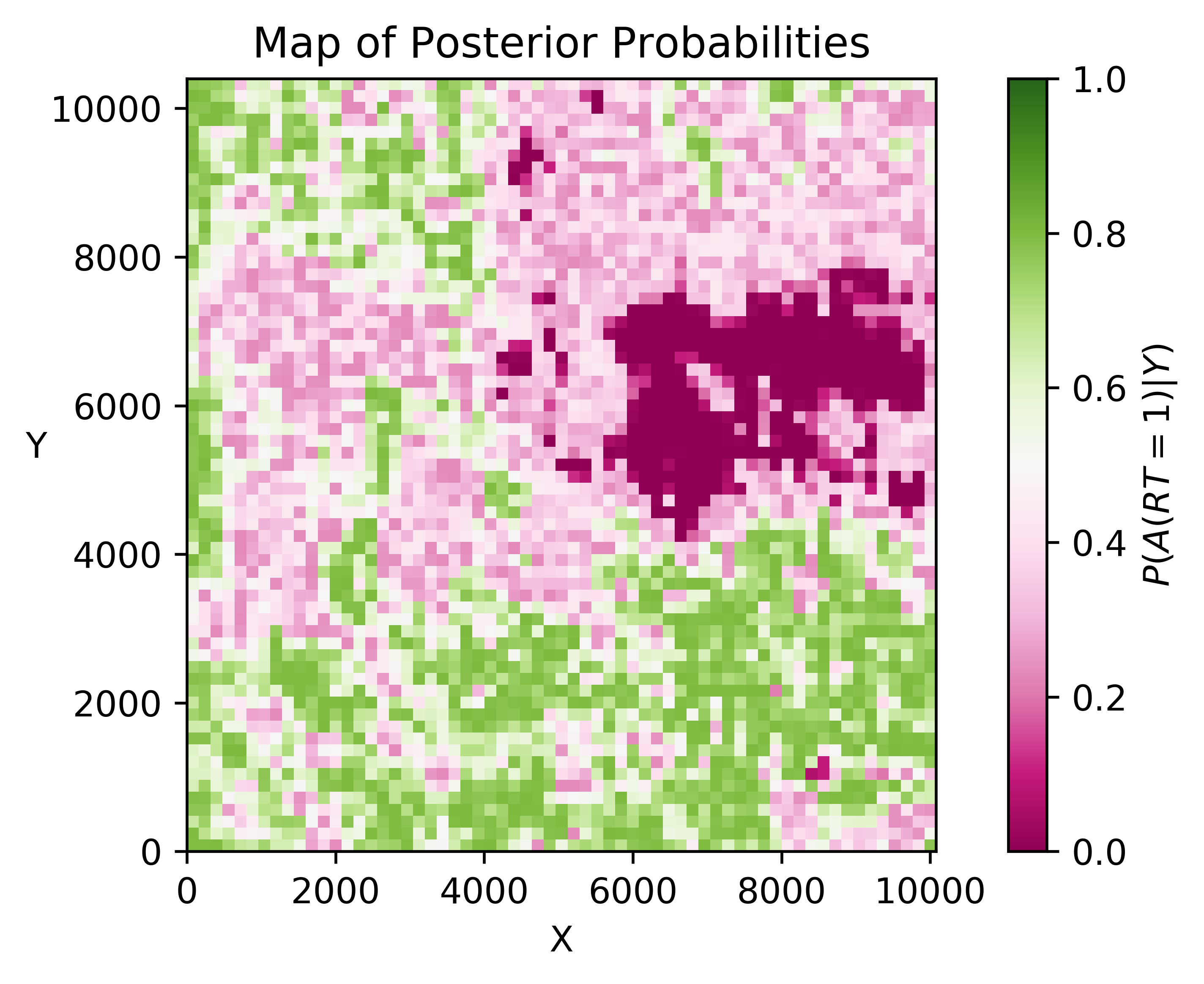
Following is a small geostatistical application of using Bayes theorem to update a prior probability \(P(A)\) to consider additional evidence or data. The inversion of \(f_{Y|A}(y)\) to the desired \(P(A|y)\) is illustrated, that is, the concept of updating a prior by a likelihood.

Implementation Details

This simple example considers a binary rock type indicator and a single secondary variable. In practice, there may be multiple rock types and multiple secondary data. There is no fundamental difference in the approach. A larger number of rock types means fewer observations of the secondary data per rock type. A larger number of secondary data means a higher dimensional likelihood distribution must be inferred. KDE is both more challenging and important for these higher dimensions.

The simple example above considers a categorical \(A\) variable being prediced. In practice, the variable being predicted could be a continuous rock property. The application of Bayes Theorem is the same, but the likelihood distribution is extracted from a multivariate distribution considering the primary and secondary. In principle, once the full multivariate distribution of all primary and secondary data is established the need for Bayes Theorem is diminished; the desired conditional distributions could be extracted directly. Consideration of local conditioning data complicates matters.

Local Conditioning

The posterior probabilities calculated above are posterior in the context of the secondary data, but there are local conditioning data that should be considered. At locations where local measurements show a rock type of 1 (not-\(A\)) or 0 (\(A\)), the probabilities must be 1 or 0 depending on the measured value. Note that the map of \(P(A({\mathbf{u}})|y({\mathbf{u}}))\) depends only on \(Y\) and not the local conditioning data. Simply resetting the posterior probability values to 0 or 1 at the data locations is not enough. There is spatial correlation evident in the rock type distribution. The probability of \(A\) will diminish from 1 gradually away from an \(A\) conditioning data; the probability of \(A\) will increase from 0 gradually away from a not-\(A\) conditioning data. Consideration of this spatial correlation is within the classic paradigm of geostatistics.

The Bayesian framework developed for the consideration of \(Y\) is not easily extended to consider \(Y\) and the local conditioning data at each location. The data configuration and \(Y\) data values around each unsampled location is different; there are no repetitions of data patterns available to calculate likelihood values for precisely the same configuration. There are many ways to address the challenge of simultaneous consideration of secondary data and spatially distributed data of the same type. Any geostatistics book can be reviewed. A simple solution will be demonstrated here.

The approach proposed here consists of three steps (1) calculate the posterior probability given the secondary data as described above, (2) calculate the probability of \(A\) given the local configuration of data relative to the unsampled location, and (3) combine the probabilities together with some function (\(\phi\)) making a reasonable assumption about the relationship between \(Y\) and the local data:

\[ P(A({\mathbf{u}})|y({\mathbf{u}}),n({\mathbf{u}})) \approx \phi (P(A), P(A({\mathbf{u}})|y({\mathbf{u}})), P(A({\mathbf{u}})|n({\mathbf{u}})) ) \;\;\; {\mathbf{u}} \in \mbox{Domain} \]

The notation \(n({\mathbf{u}})\) refers to the neighborhood of direct measurements relevant to location \({\mathbf{u}}\) consisting of some number of data, the data locations and the rock types at those locations. The notation \(\phi\) refers to a function to combine the two different conditional probabilities; this comes later.

There are a number of options for the inference of \(P(A({\mathbf{u}})|n({\mathbf{u}}))\) for all locations \({\mathbf{u}} \in\) Domain. The most direct approach would be to find replicates of the \(n+1\) events, that is, the configuration of \(n({\mathbf{u}})\) data plus the unsampled location. Then, the conditional probability could be calculated directly by the proportion of times \(A\) was observed given \(n({\mathbf{u}})\). This is the Multiple Point Statistics (MPS) technique in geostatistics. MPS requires a large database of patterns called a training image. If a reliable training image is not available, then indicator kriging (IK) could be performed using a covariance model for the indicator random function. This approach will be taken here.

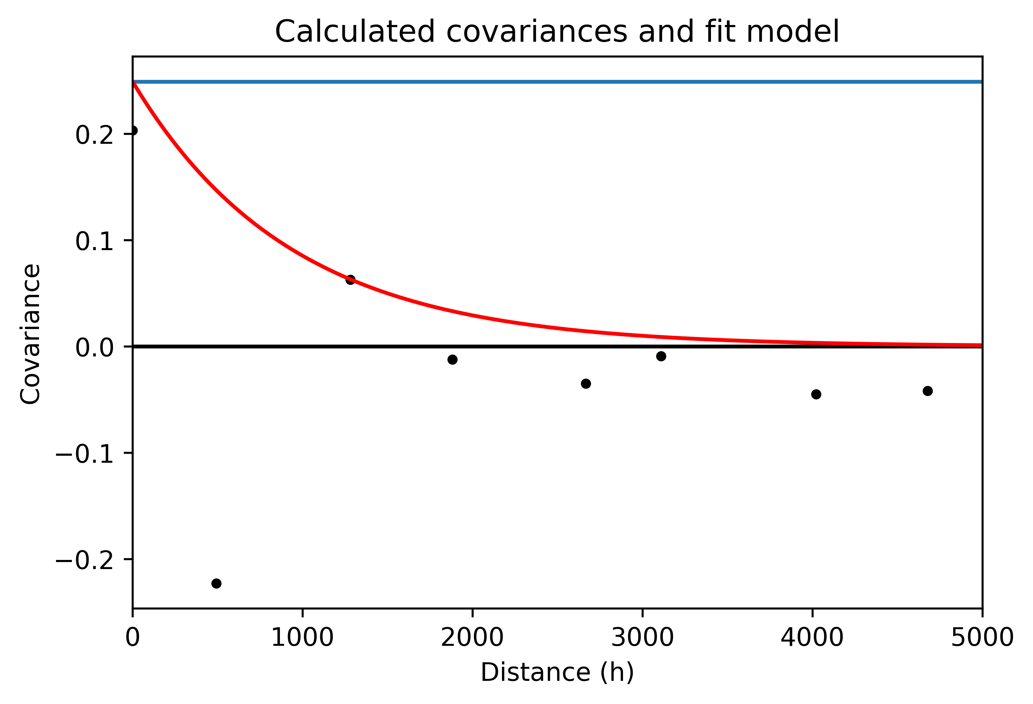
The details of infering covariance/variogram functions and indicator kriging are found in many geostatistical references. A simplified implementation is provided here. Consider the deemed stationary indicator regionalized variable \(A({\mathbf{u}})|n({\mathbf{u}}))\) for all locations \({\mathbf{u}} \in\) Domain with mean value \(E\{A({\mathbf{u}})\}=p=0.528 \forall\) locations \({\mathbf{u}} \in\) Domain. The covariance between two locations is also considered stationary, that is, it only depends on the separation vector \({\mathbf{u}}\) between the locations: \(C({\mathbf{u}},{\mathbf{u}+h})\) = \(C({\mathbf{h}})\) = \(E\{ A({\mathbf{u}}) \cdot A({\mathbf{u}}+{\mathbf{h}}) -p^2 \}\) \(\forall\) locations \({\mathbf{u}} \in\) Domain. For the sake of simplicity we assume that the covariance is isotropic (depends only on distance and not direction) and can be modeled by an exponential function. Experimental pairs averaged within distance classes and the covariance model are shown. The experimental covariance is strongly negative at the first lag due to the unique data configuration, and is not used when fitting the covariance model.

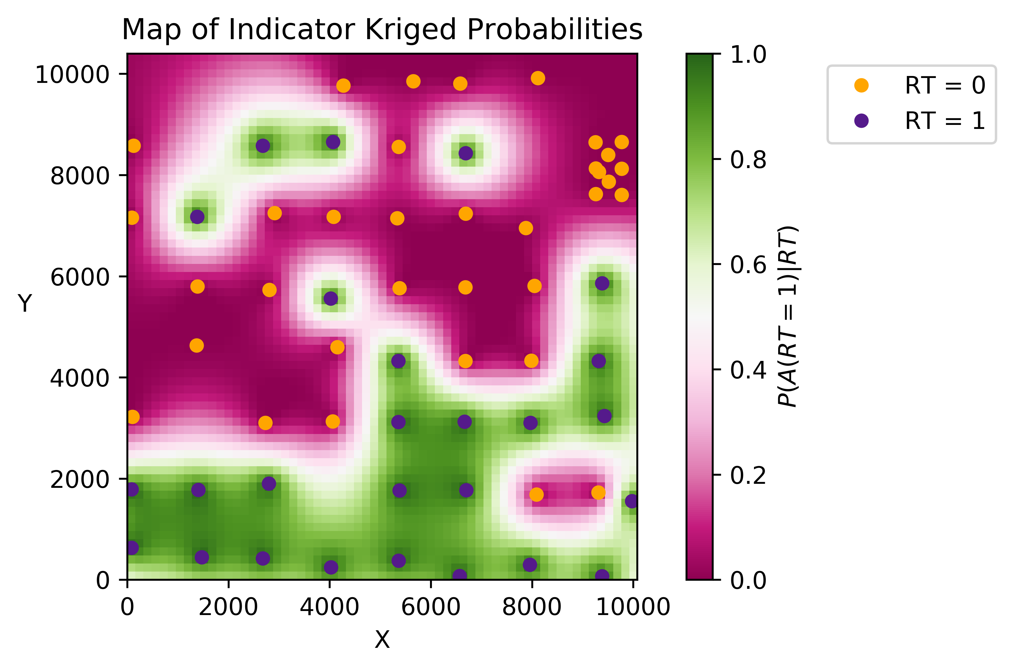
The probability of \(A\) at each unsampled location can be calculated from the data with indicator kriging, that is, estimating the event \(A\) at each unsampled location using a linear estimator with a minimum mean squared error criterion. A constraint that the weights sum to one is considered to avoid dependence on the global mean. The kriging or regression equations are solved in their dual form for efficiency. Define \({\mathbf{a}}^T\) = \([a_1, \ldots, a_n, 0]\) as the vector of conditioning data (plus a zero), \({\mathbf{c}}^T\) = \([C({\mathbf{u}},{\mathbf{u}}_1), \ldots, C({\mathbf{u}},{\mathbf{u}}_n), 1]\) as the vector of the covariance between each data and the unsampled location \({\mathbf{u}}\) (plus a one), and \({\mathbf{C}}(i,j)=C({\mathbf{u}}_i,{\mathbf{u}}_j)\) for \(i,j=,\ldots,n\) and \({\mathbf{C}}(n+1,i)\) = \({\mathbf{C}}(i,n+1)\) = 0 for \(i=1,\ldots,n\) and \({\mathbf{C}}(n+1,n+1)\) = \(1\). The estimated probability of \(A\) at each unsampled location is given by the global dual ordinary indicator kriging equations:

\[ P(A({\mathbf{u}})|n({\mathbf{u}})) \approx {\mathbf{C}}^{-1} {\mathbf{a}} {\mathbf{c}} \;\;\; {\mathbf{u}} \in \mbox{Domain} \]

Note that only the last term \({\mathbf{c}}\) depends on the unsampled location, thus \({\mathbf{C}}^{-1} {\mathbf{a}}\) is solved only once and is referred to as the dual kriging weights. Note also that the estimate is not guaranteed to be within 0 and 1 as it must; these constraints are imposed after estimation. The local probabilities are calculated and shown below:

Now, back to the function to combine the two conditional probabilities (\(\phi\)). A common one in geostatistics is called permanence of ratios (Journel, 2002). There are variations on this model in the geostatistics literature and various probabilistic classifiers in machine learning that are similar. The permanence of ratios combination function for two data sources is given by:

\[ \phi ( P(A), P(A|B), P(A|C) ) = \frac{ \frac{1-P(A)}{P(A)} } { \frac{1-P(A)}{P(A)}+\frac{1-P(A|B)}{P(A|B)} \cdot \frac{1-P(A|C)}{P(A|C)} } \]

where \(A\) is \(A({\mathbf{u}})\), \(B\) is \(y({\mathbf{u}})\), \(C\) is \(n({\mathbf{u}})\) and this is applied for all locations \({\mathbf{u}} \in\) Domain:

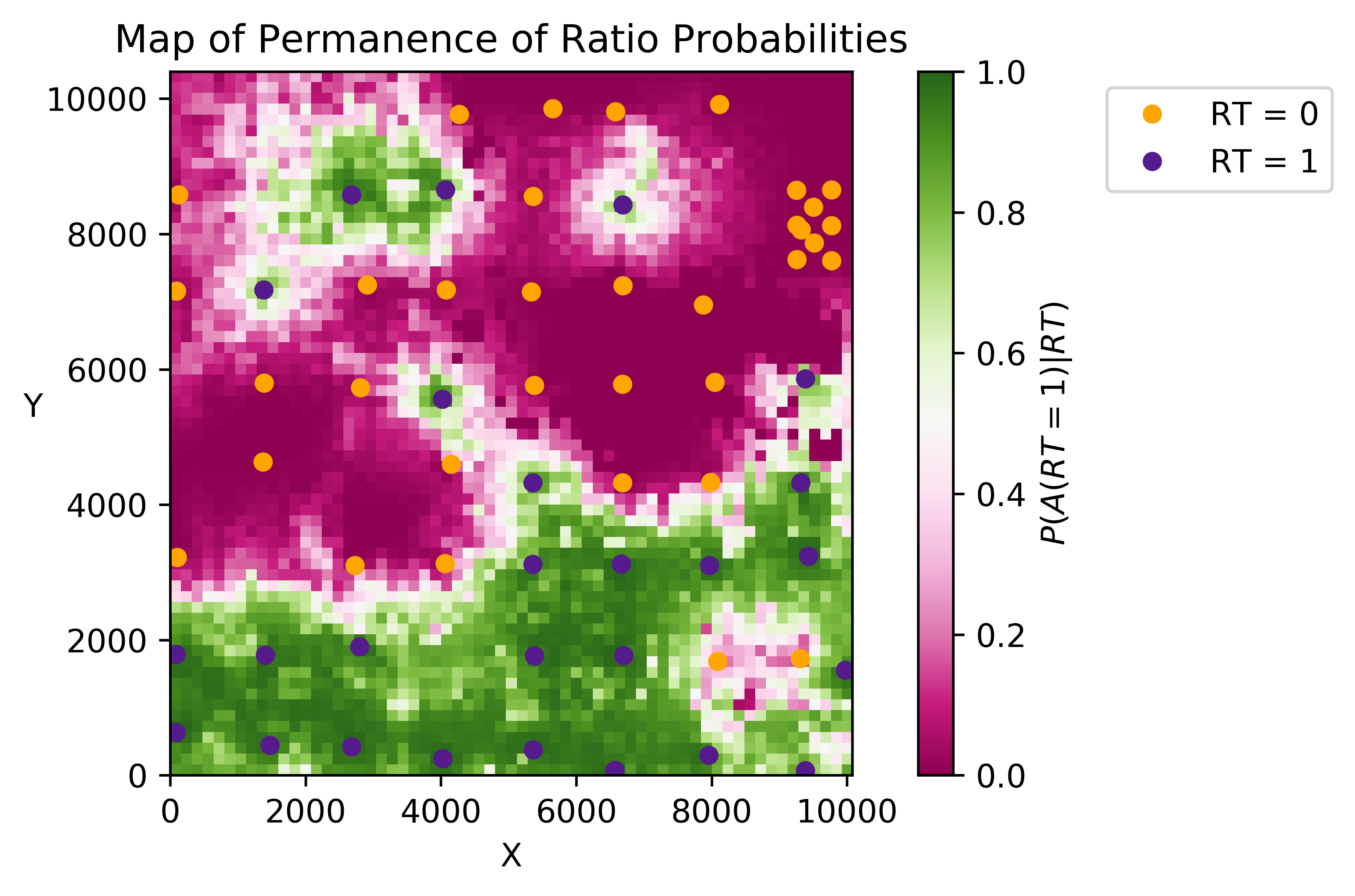
The result considers the secondary data and direct measurements of $A%. Note that there are more areas where the probabilities are closer to 0 and 1: areas identified by the secondary data and areas identified by the direct measurements. The uncertainty at unsampled locations has been reduced. The only way to reduce the uncertainty further is to consider additional data.

There are alternatives in geostatistics for data integration including cokriging, but this presents a reasonably straightforward implementation for geostatistical mapping. The uncertainty quantified above is for each location one at a time, which is suitable for many purposes. The simultaneous uncertainty of multiple locations at a time is required for some applications and this uncertainty would have to be sampled by simulation, for example, a sequential simulation procedure.

Summary

The notion of Bayesian inversion is important for geostatisticians. The posterior conditional probability of our variable of interest given secondary data is proportional to the prior global probability of the variable of interest and the likelihood probability of the secondary data given the variable of interest. In the presence of relatively few direct measurements it is relatively straightforward to infer the likelihood distributions, then apply Bayesian inversion. The notion of conditioning is important for statisticians. The local configuration of data around each unsampled location is unique and defies a straightforward application of Bayes Theorem. Indicator kriging is one approach to estimate the conditional probability of an event at an unsampled location given surrounding conditioning data. Combining two estimates of conditional probability can be made with permanence of ratios. There are other ways to approach this problem, but the variety of principles touched on in this Lesson are important and widely used throughout geostatistics.

References