Learning Objectives

• Review variogram estimators.
• Appreciate the behavior of the pairwise relative variogram.
• Understand the sill and potential bias of the pairwise relative variogram.
• Understand the techniques and comparisons (source code available).

Introduction

A characteristic of geostatistics is that spatially dependent data are encountered in modeling. Data values that are close are more likely to be similar. As a result, before estimation or simulation, understanding this spatial dependency is a crucial step. The pairwise relative variogram is one estimator of the variogram (David, 1988).

The variogram is a geostatistical tool to characterize spatial dependency. The traditional experimental variogram is often unstable due to sparse data with outliers and clustered data with a proportional effect (David, 1988). As a result, various robust variograms have been proposed including the correlogram and normal score variogram (Isaaks & Srivastava, 1989). Among the alternatives, the pairwise relative variogram is a very stable estimator. The pairwise relative variogram was proposed by Michel David in 1977 (Deutsch & Journel, 1997). The idea came from standardizing the experimental traditional variogram with locally changing variance of the data (David, 1988). There are two concerns about the pairwise relative variogram. The first is that, until recently, the sill of the pairwise relative variogram was not fully understood. Thus, it was hard to interpret and model the variogram. The second is that the pairwise relative variogram is not theoretically correct. The first problem can be solved by simulation. For the second, it is shown that although the pairwise relative variogram is not theoretically correct, it converges to the true variogram when we have large data sets (Wilde & Deutsch, 2006).

Variogram estimators for different examples are presented to show that the pairwise relative variogram can overcome the problems of sparse data with outliers and clustered data with the proportional effect. The sill of the pairwise relative variogram and the convergence to the true variogram are also addressed.

Variogram and Variogram Estimators

The regionalized variable \(\left\{Z\left(\mathbf{u}\right)\text{,}\mathbf{u}\in\mathbf{A}\right\}\) can be considered with a lag vector \(\mathbf{h}\). The variogram \(2\gamma\left(\mathbf{h}\right)\) is the variance of the data for lag vector \(\mathbf{h}\):

\[ 2\gamma\left(\mathbf{h}\right)=E\left\{\left(Z\left(\mathbf{u}\right)-Z\left(\mathbf{u}+\mathbf{h}\right)\right)^2\right\} \]

The variogram measures how dissimilar the variable is for different lag vectors. When the lag distance increases, the dissimilarity of the variable will likely increase.

Traditional Experimental Variogram

The variogram can be estimated by the experimental variogram, which is defined as the average of the squared difference of the variable at two locations. It is an unbiased estimator to the variogram. The experimental variogram can be calculated as (Deutsch & Journel, 1997):

\[ \gamma_{Exp}\left(\mathbf{h}\right)=\frac{1}{2N(\mathbf{h})}\sum_{i=1}^{N(\mathbf{h})}{(Z(\mathbf{u}_{i})-Z(\mathbf{u}_{i}+\mathbf{h})})^2 \]

where \(N(\mathbf{h})\) is the number of pairs of data separated approximately by lag distance \(\mathbf{h}\).

Problems with the Experimental Variogram

Calculating a stable experimental variogram is sometimes difficult (Isaaks & Srivastava, 1989). The first difficulty is sparse data with outliers. When the data is sparse, the pairing process can lead to unequal pairing of the outliers; the outliers are included a different number of times in different lags. This leads to noise in the variogram. The second difficulty is the proportional effect. In mining and petroleum applications, it is common to have more data samples in high-valued areas. Furthermore, the data with higher values usually have higher variance. This phenomenon is called the proportional effect (Manchuk, Leuangthong, & Deutsch, 2007). As a result, the shorter distance lags usually have a higher variance. These two major reasons cause the experimental variogram to be noisy and unstable.

Alternatives to the Traditional Experimental Variogram

As a result, there is a need to improve the experimental variogram. Many robust variograms have been proposed (Chilès & Delfiner, 2012). One approach is to use different measures such as the madogram (absolute value of the difference) and rodogram (absolute difference to the power of 0.5) (Chilès & Delfiner, 2012). Another approach is the normal score transformation or log-transformation. Other alternatives to the traditional experimental variogram are the correlogram, the pairwise relative variogram, and the back transformed normal score variogram (Wilde & Deutsch, 2006).

Correlogram

The covariance \(C(\mathbf{h})\) of the paired values at \(\mathbf{u}\) and \(\mathbf{u}+\mathbf{h}\) can be calculated. The covariance can be standardized to get the correlation with respect to the lag distance \(\mathbf{h}\). In general, the larger the lag distance \(\mathbf{h}\), the smaller is the correlation. The measure one minus the correlation would look like a variogram and is called the correlogram. The correlogram can be calculated by the following (Deutsch & Journel, 1997):

\[ \gamma_{Corr}\left(\mathbf{h}\right)=1-\frac{C\left(\mathbf{h}\right)}{\sigma_{Z\left(\mathbf{u}\right)}\sigma_{Z\left(\mathbf{u}+\mathbf{h}\right)}} \] \[ C\left(\mathbf{h}\right)=\frac{1}{N\left(\mathbf{h}\right)}\sum_{i=1}^{N\left(\mathbf{h}\right)}Z\left(\mathbf{u}_i\right)Z\left(\mathbf{u}_i+\mathbf{h}\right)-m_{Z\left(\mathbf{u}\right)}m_{Z\left(\mathbf{u}+\mathbf{h}\right)} \]

where \(m_{Z(\mathbf{u})}\) is the mean of the attribute value Z at the location \(\mathbf{u}\), \(m_{Z(\mathbf{u}+\mathbf{h})}\) is the mean of the attribute value Z at the location \(\mathbf{u}+\mathbf{h}\), \(\sigma_{Z(\mathbf{u})}\) is the standard deviation of the attribute value Z at the location \(\mathbf{u}\), and \(\sigma_{Z(\mathbf{u}+\mathbf{h})}\) is the standard deviation of the attribute value Z at the location \(\mathbf{u}+\mathbf{h}\). These mean and standard deviation values change for each lag distance \(\mathbf{h}\). The correlogram is relatively robust with respect to outliers and clustered data; however, there may be concerns in presence of trends or zonal anisotropy.

Normal Score Transformed Variogram

The data is transformed to a standard normal distribution. As a result, the outliers and the proportional effect are eliminated. Then, the experimental variogram is used to calculate the normal score variogram. Finally, the variogram can be back transformed from normal score space into the variogram of original unit using hermite polynomials or simulation, see (Wilde, Neufeld, & Deutsch, 2007) or the Lesson “Transforming a Variogram of Normal Scores to Original Units”. This measure is also robust with respect to outliers and clustered data.

The Pairwise Relative Variogram

The proportional effect is common with positively skewed geological data. The higher data values have a higher variance. The experimental variogram could be standardized by the local mean of the data, trying to mitigate the proportional effect (David, 1988). For the general relative variogram, the traditional experimental variogram is adjusted by dividing by the squared mean of the data used for each specific lag distance \(\mathbf{h}\) (David, 1988). The pairwise relative variogram considers the mean for each data pair. The squared average of the data enters the denominator. The pairwise relative variogram is calculated as (Deutsch & Journel, 1997):

\[ \gamma_{PR}\left(\mathbf{h}\right)=\frac{1}{2N\left(\mathbf{h}\right)}\sum_{i=1}^{N\left(\mathbf{h}\right)}\left(\frac{Z\left(\mathbf{u}_i\right)-Z\left(\mathbf{u}_i+\mathbf{h}\right)}{\frac{Z\left(\mathbf{u}_i\right)+Z\left(\mathbf{u}_i+\mathbf{h}\right)}{2}}\right)^2 \]

The pairwise relative variogram is usually more stable than the traditional variogram. When an outlier is encountered in the pair, the variogram value will be divided by a higher mean value, making it more stable. When the proportional effect is encountered, dividing by the mean can reduce the variance of high valued data. The pairwise relative variogram is for strictly positive variables; zero values should be reset to an arbitrarily low constant value.

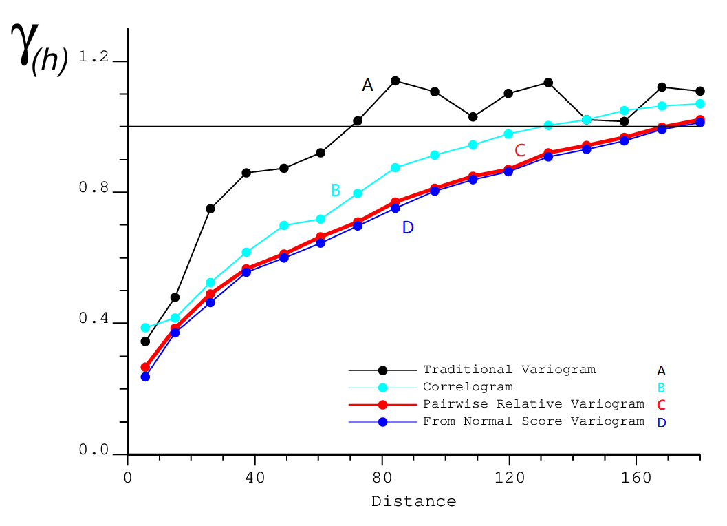
Practical application has shown that the pairwise relative variogram is very stable. The following example is from copper grades from a porphyry deposit. There is a strong proportional effect and clustering of the data in this deposit (Black: Traditional Experimental Variogram; Red: Pairwise Relative Variogram; Light Blue: Correlogram: Dark Blue: Normal Score Transformed Variogram). Both the pairwise relative variogram and the normal score back transformed variogram are equally stable. They are more stable than the traditional experimental variogram.

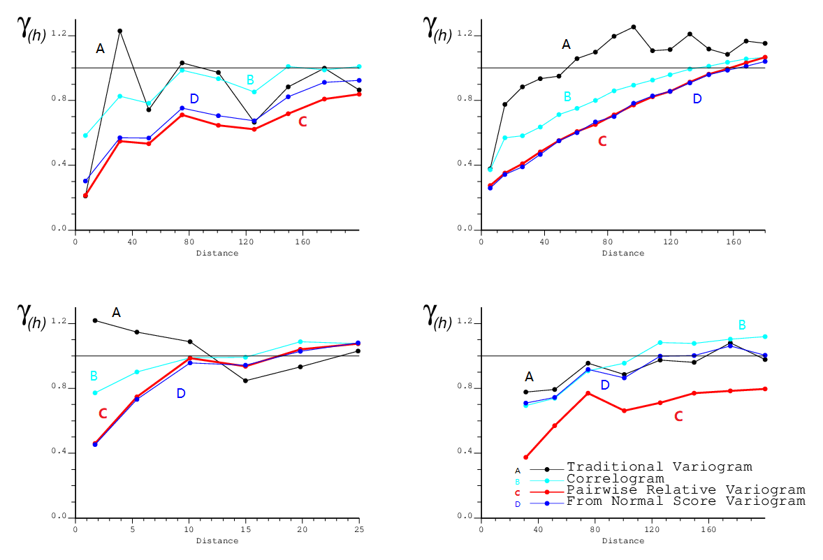
The pairwise relative variogram can behave differently in different scenarios. Four examples are shown below to illustrate different effects due to different configurations of data and different variables.

In the top left corner, the data are copper grades from a skarn deposit. The experimental variogram is very unstable because of outliers in the data. In the top right corner, the data are gold grades from a porphyry deposit. The overall trend is represented by all variograms, but the pairwise relative variogram and normal score back transformed variogram are very stable. In the bottom left corner, the pairwise variogram behaves slightly better than the experimental variogram. The three alternatives of the experimental variograms are more stable than the experimental variogram at short distances. In the bottom right corner, the data are fluorite grades from a skarn deposit. The overall configuration of all the variograms are similar. The pairwise relative variogram is consistently more stable than the other three, which means that the pairwise relative variogram may be a better experimental measure.

The Problems of The Pairwise Relative Variogram

The pairwise relative variogram can be very stable and easier to interpret and model. However, there are two major problems. One is that the sill of the pairwise relative variogram is not easily calculated. The other is that the pairwise relative variogram is not correct in theory, and may not converge to the correct value.

The Sill

The sill is important in interpreting and modeling variograms. Cyclicity, trends, anisotropy and other geological structural features benefit from knowing the sill (Isaaks & Srivastava, 1989). The sill of the traditional experimental variogram is the variance of the data. Furthermore, the sill of the correlogram and the normal score variogram can be easily standardized to be one. However, the denominator used to standardize the pairwise relative variogram changes the sill. There are three factors that influence the sill of the pairwise relative variogram: the mean, the variance, and the shape of the distribution. The sill is related to the coefficient of variation (Babakhani & Deutsch, 2012), yet there is no simple way to predict the sill of the pairwise relative variogram from summary statistics.

The sill could be calculated by Monte Carlo simulation. The empirical cumulative distribution function of the data is calculated. Then, many data pairs are drawn randomly from the distribution. The pairwise relative variogram calculated from the random pairs is the sill. This straightforward approach to calculate the sill could easily be used in variogram calculation software.

Potential Bias

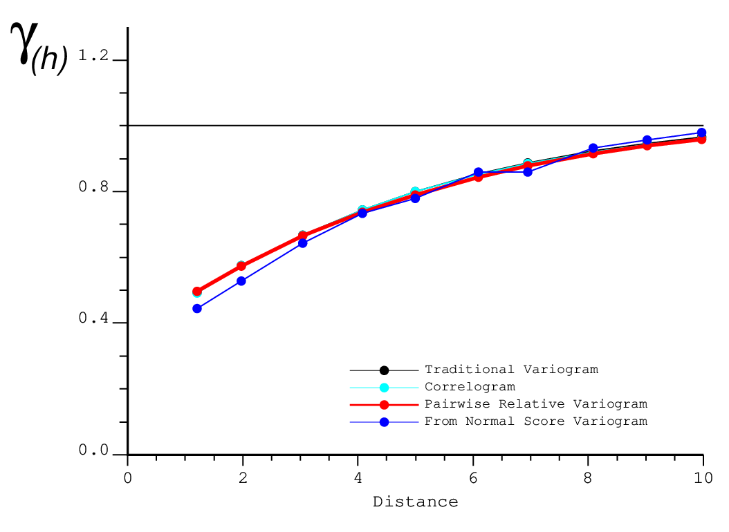
The pairwise relative variogram is theoretically incorrect. However, it has been shown that if exhaustive data are available, the pairwise relative variogram will be very close to the true variogram (Wilde & Deutsch, 2006). Here, another example shows this property. Data with a lognormal distribution (mean = 1, standard deviation = 2) are simulated on a 512 by 512 grid. In the following figure, it can be seen that all four variogram estimators are very close to each other. Many other experiments like changing the distribution and the variogram have been done in order to make sure that the result is universal. Thus, the pairwise relative variogram can be used as a tool to conduct structural analysis.

Discussion and Summary

The pairwise relative variogram can be a very stable estimator to the experimental variogram. It can mitigate the noise caused by sparse data with outliers and clustered data with the proportional effect. The sill of the pairwise relative variogram can be calculated by simulation which facilitates interpretation. Also, although the pairwise relative variogram is not theoretically correct, it reasonably converges to the variogram. We are not concluding that the pairwise variogram should be used in all circumstances. The correct measure is the experimental variogram or covariance of the data that will be entering kriging or simulation. If the experimental variogram is noisy or unstable, then we could consider alternative measures including the pairwise relative variogram. A more robust alternative may be closer to the true variogram.

References