Learning Objectives

• Recognize the importance of accounting for local variations in anisotropy to improve variogram based geostatistical modeling
• Review how variogram based modeling methods are modified to incorporate LVA
• Understand how different data sources can be used for the construction of the LVA field
• Appreciate the difference between LVA and ‘dynamic anisotropy’

Introduction

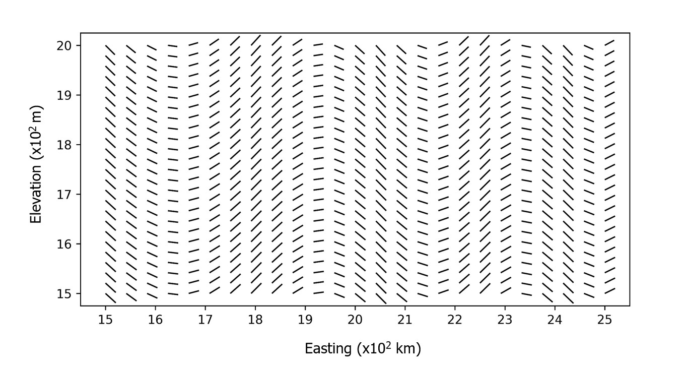
All modeling techniques rely on a decision of stationarity (Dias & Deutsch, 2022). In most geostatistical algorithms, this is (1) first order stationarity: the global mean is constant in the modeling domain and (2) second order stationarity: the spatial continuity of the random function is unchanged under translation. This lesson explores modeling geological domains where second order stationarity is inappropriate and spatial continuity/anisotropy varies locally, termed locally varying anisotropy (LVA), Figure 1. Note that when only considering the direction of anisotropy, this is sometimes called ‘dynamic anisotropy’ but the term LVA is general and encompasses dynamic anisotropy, so the term LVA is preferred.

Spatial properties of earth science data vary depending on the direction being considered; this is known as anisotropy. Anisotropy arises due to a variety of factors including preferential alignment of geological structures and differences in the properties of different geological processes. This can pose a challenge to many geostatistical techniques when the magnitude or direction of that anisotropy varies within a modeling domain. Accounting for anisotropy in numerical models requires careful consideration of the direction and magnitude of anisotropy, and requires the use of specialized methods that account for LVA when domains are non‐stationary.

Most geostatistical workflows can be modified to consider a non‐stationary framework and this lesson focuses on Kriging and Sequential Gaussian Simulation (SGS). Non‐stationary modeling considers a trend in the mean or a trend in the covariance function (Honarkhah & Caers, 2012); thus, LVA is just a ‘trend in the variogram’ and is characterized by a location‐dependent covariance structure (Ejigu, Wencheko, Moraga, & Giorgi, 2020), demonstrated in Figure 1. LVA typically improves estimation by accounting for local features in a modeling domain and generates models that are more geologically realistic, but requires additional inputs to define the locally varying covariance structure.

What is LVA?

A single stationary variogram with a constant strike/dip/plunge and constant ranges in each direction cannot represent local variations in continuity typical of mineral deposits. LVA parameterizes the spatial continuity of a domain using a vector field (Figure 2) that represents the covariance function (i.e. variogram) in a domain. Models generated using LVA usually exhibit greater geological realism, meaning they include characteristics that are more representative of natural geological systems.

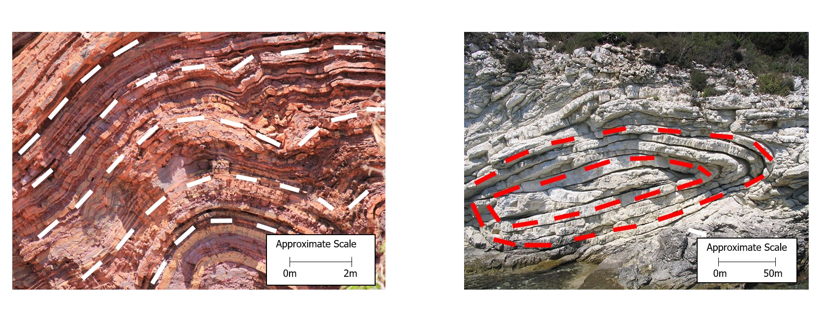
The LVA field is a vector field parameterized by six parameters (Lillah & Boisvert, 2015). A detailed discussion and description of the dynamic representation of anisotropy is provided in Lesson (Deutsch, 2015). The six parameters that define anisotropy are: the strike (α) is the angle measured from the geographic north to the horizontal plane; the dip (β) is the largest acute angle measured between the horizontal and the bedding plane; the plunge (θ) is the angle between the horizontal and the linear structure; the major; minor (also referred to as semi) and vertical (also referred to as minor) directions of continuity. An ‘LVA field’ is the specification of these 6 values for every location in a model. \(r1\) is the ratio between ranges along the minor and major directions of continuity; \(r2\) is the ratio between the ranges along the vertical and major directions of continuity. The LVA field can be defined using more than one variogram structure by specifying the ranges and angles for each structure when software allows. The LVA field is used to calculate the covariance between locations, just as the variogram is used in traditional modeling workflows.

Spatial Modelling Methods with LVA

The options for integrating LVA into geostatistical modeling are reviewed. The simplest method is to consider stationary modeling/estimation domains for anisotropy variations having hard boundaries (Boisvert, 2010). The second method considers a local reorientation of the variogram and has been popular since the 1990s; this remains a good methodology when the LVA in a domain varies at a scale larger than the sample spacing (David F. Machuca-Mory & Deutsch, 2007). When there is significant variation in anisotropy at the sample spacing scale, the third workflow involving calculating shortest path distances (SPD) is appropriate (Boisvert & Deutsch, 2011). Note that all of these methods are appropriate for nearly any variogram based geostatistical technique.

Hard Boundary Between Domains

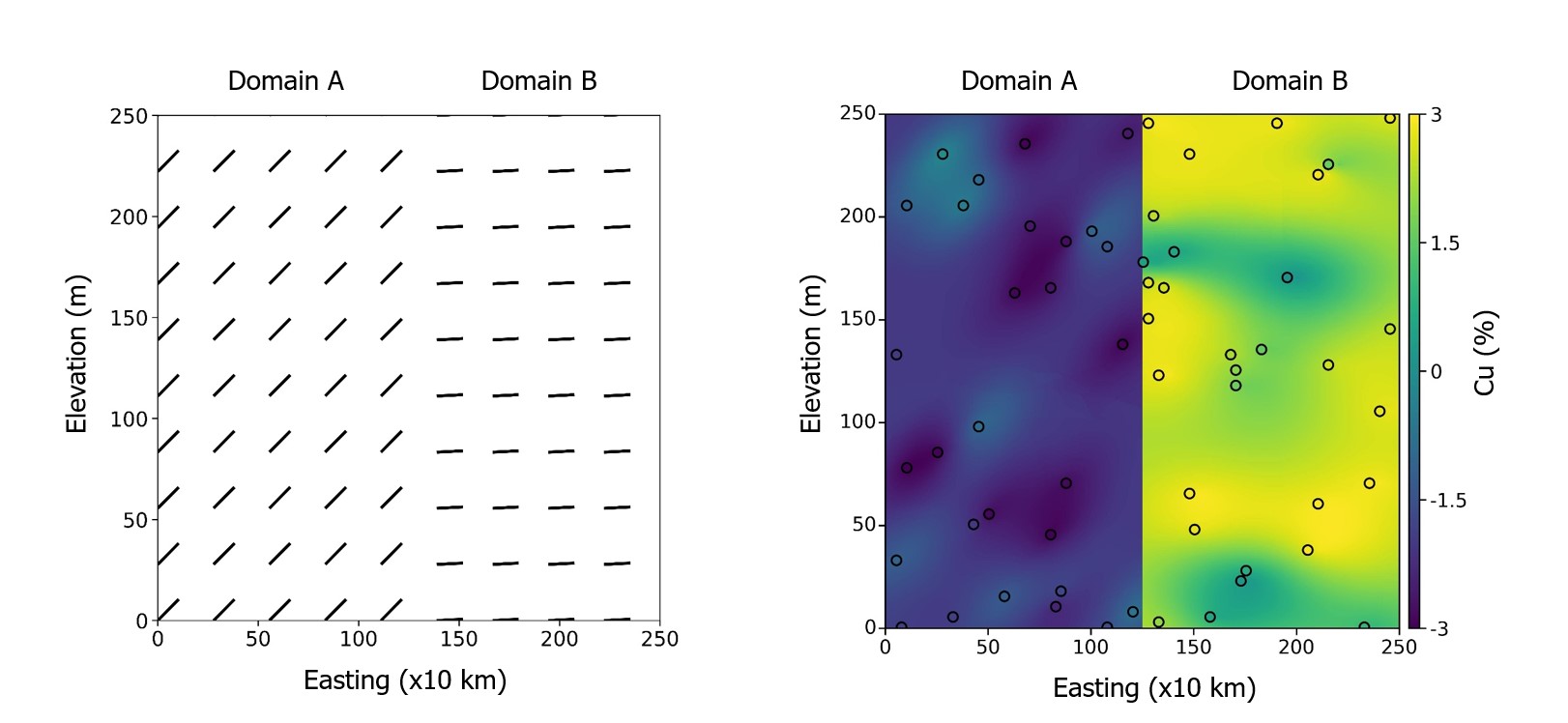
This method is simple, when the LVA changes abruptly and a hard boundary can be drawn between domains with constant anisotropy (i.e. Domains A and B in Figure 4) multiple estimation domains should be considered (Boisvert, 2010). This is the preferred workflow when a hard boundary delineates a large volume of the domain of interest and there is sufficient sampling in all domains to infer the necessary parameters required for modeling (i.e., histogram, variogram, categories, etc). Referring to Figure 3 as ‘locally varying’ is a stretch, but the method is included here for completeness.

Local Reorientation of the Variogram

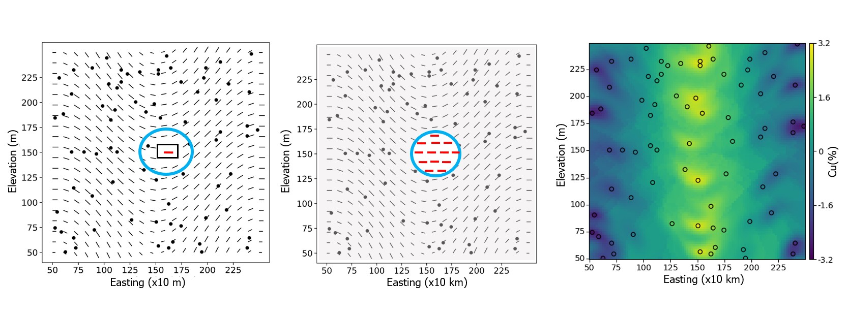
When considering LVA in geostatistical modeling, it is essential to address the relative scale of anisotropy changes compared to sample spacing. This concept is particularly pertinent when discussing the local reorientation of the variogram. In this methodology, the covariance function at the location being estimated or simulated is used and applied to the local estimation neighborhood (Kupfersberger, Deutsch, & Journel, 1998; David F. Machuca-Mory & Deutsch, 2007). This local estimation neighborhood or the ‘search’ radii is typical in most software implementations. The covariance between all samples and previously simulated nodes in this search volume is required. The local variogram reorientation methodology uses the anisotropy at the estimation location and assumes it is constant in the local search neighborhood. Sufficient sampling in all domains is required to infer the necessary parameters for modeling (i.e., histogram, variogram, categories, etc). Once these required covariances are calculated, Kriging or simulation proceeds as in traditional workflows. This is appropriate for domains where continuity varies smoothly and at a scale larger than the data spacing. However, the effectiveness of this technique can be compromised if the samples are spaced widely relative to the scale of anisotropy changes. In such cases, the assumption of constant anisotropy within the local search neighborhood may not hold, leading to potential inaccuracies in the model predictions (David F. Machuca-Mory, Rees, & Leuangthong, 2015).

Shortest Path Distance for LVA

Locally reorienting the variogram cannot consider anisotropy that varies within the local search neighborhood so the covariance between locations must be modified to consider LVA (Figure 5). One popular workflow is to consider the shortest path distance (SPD) between locations and use this to calculate the covariance accounting for the ‘correct’ relationship between points(Boisvert & Deutsch, 2011). Consider two locations A and B in Figure 6. It is clear that these locations are not related by the straight‐line Euclidean path A‐B; rather, during deposition A and B would have been parallel and in their current orientation they would be related by the curved path shown. Interestingly, when the underlying LVA field is used to calculate the anisotropic distance, the curved path is shorter than the straight‐line path because of the discounting of distance when following ‘along’ the direction of continuity. When calculated, the curved SPD is 27% shorter than the straight‐line path, meaning that the use of the Euclidean straight‐line distance underestimates how correlated A and B are. The detailed calculation for SPD can be found in Boisvert & Deutsch (2011).

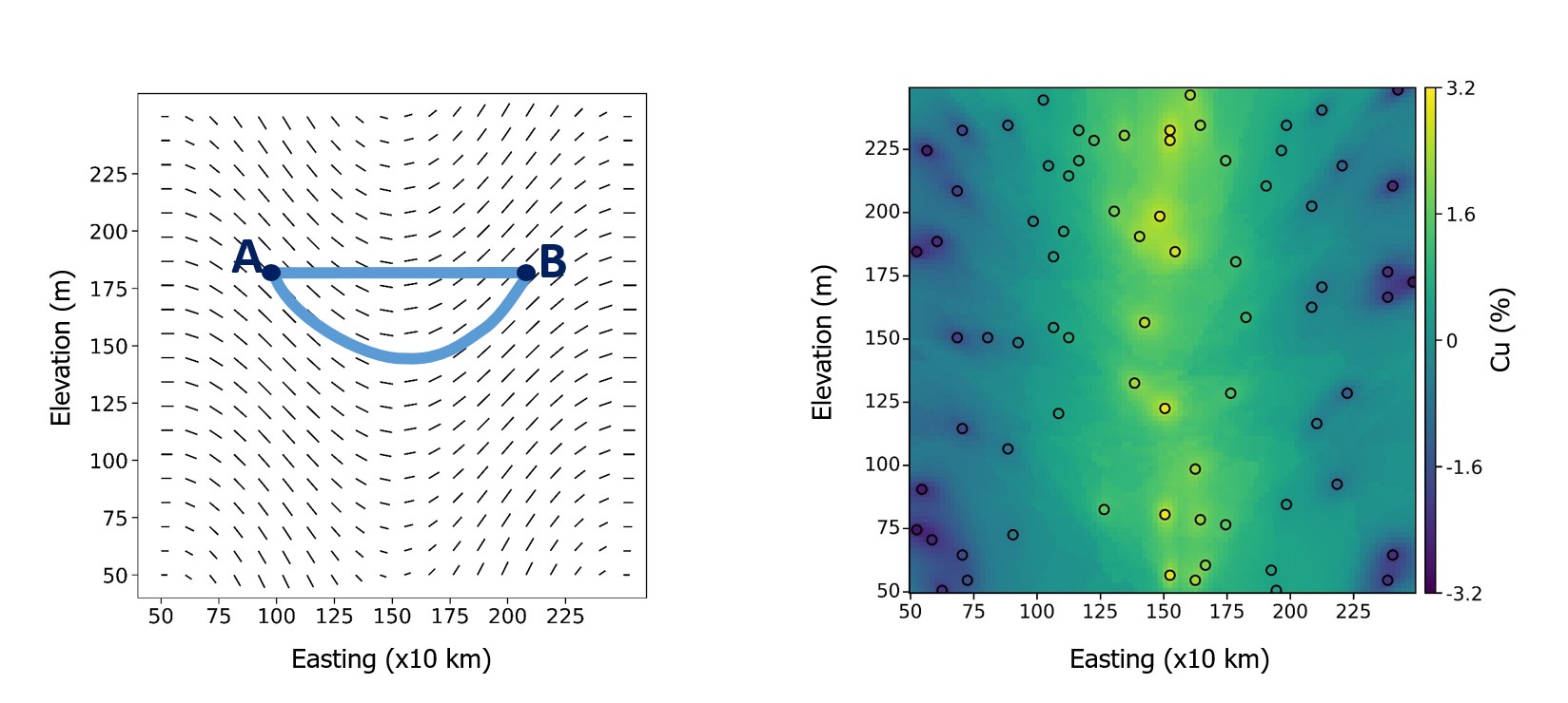
Different implementations of this workflow calculate this SPD in different ways. Using a graph and the Dijkstra algorithm is one method (Boisvert, Manchuk, & Deutsch, 2009). The path is considered to be piecewise linear segments that make up a graph and distances of each segment are calculated with the local anisotropy specification from the LVA field. Any shortest path algorithm could be applied. Additional details can be found in (Bogrash, Sacchi, & Boisvert, 2023; Boisvert & Deutsch, 2011; Davis & Curriero, 2019) but the actual calculation of the SPD is usually handled well by software.

One important detail in these SPD workflows is that non‐Euclidean distances cannot be directly used in kriging equations, as the resulting system of equations are not guaranteed to be solvable. Two popular fixes are (1) adjust the resulting covariance matrix until it is positive definite (Davis & Curriero, 2019) and (2) use multidimensional scaling (MDS) to embed the samples in a high dimensional space in which Euclidean distances are appropriate (Boisvert & Deutsch, 2011) and model an omni-directional variogram for covariance calculation between samples. To date, there are no computationally efficient workflows for option 1 because it requires the calculation of many more SPD’s than option 2; thus option 1 is limited to very small 2D problems. As SPD algorithms and computational speed continues to improve, option 1 may become viable for larger grids. The use of MDS in option 2 reduces the number of SPD’s required and is computationally efficient for large 3D grids with millions of cells; however, it introduces some bias to the distance calculations, especially for short distances. Details of the landmark MDS algorithm typically employed in these workflows can be found in (Boisvert & Deutsch, 2011) but this requires very few user inputs and is handled well by software.

Example

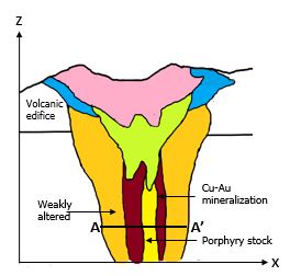
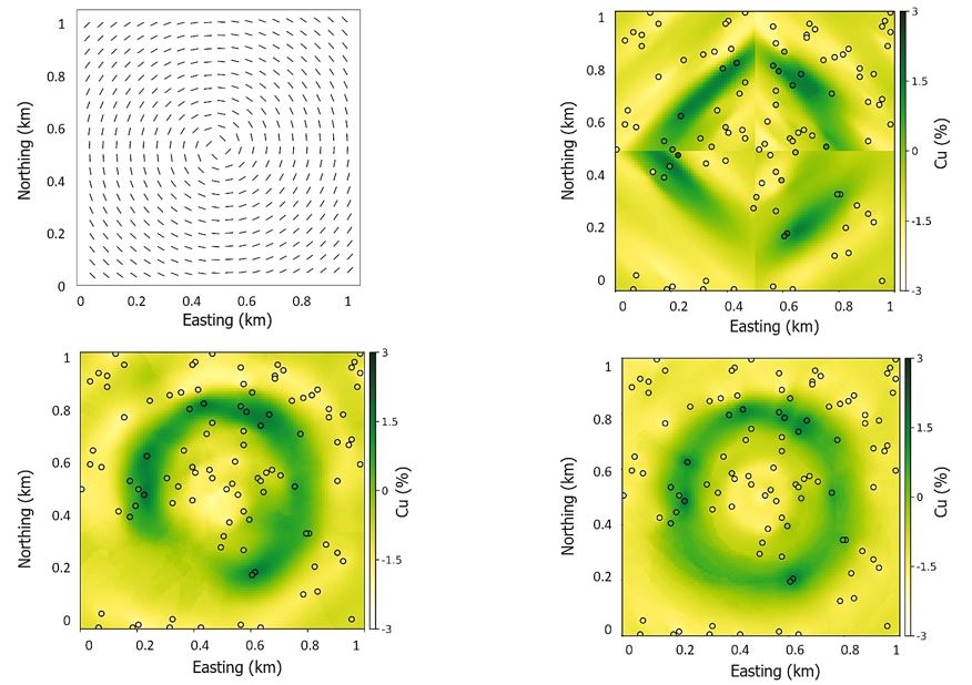
A synthetic Cu‐Au porphyry deposit (Figure 6) is used to highlight the importance of LVA in reproducing nonlinear features in geostatistical models. The LVA field for the given deposit (Figure 7) varies between the samples so SPD should be considered, but all methods are applied for comparison. It is difficult to subdomain this example into stationary domains, considering four quadrants is not sufficient (Figure 8). Some models built for similar deposits have been successful with more divisions, think of further dividing this domain into pizza slices, but that requires dense drilling so that there are sufficient samples informing the histogram and variogram for each domain. The features of the porphyry are best replicated with the SPD method (Figure 8). Considering local variogram reorientation (Figure 7) performs well in areas with dense drilling but poorly in the Southwestern area of the domain where data is sparse. As discussed, the SPD method is preferred when the LVA field varies between samples.

Building LVA Field

Building the LVA field is the most difficult part of modeling with LVA and could be the topic of a dedicated lesson, but three possible methods are briefly presented here. Selection of the LVA field generation method depends mostly on the type of data available. One method is presented for generation from surfaces (e.g. sedimentary deposits), point data (e.g. dipmeter data or hand placed angles), and exhaustive secondary data (e.g. seismic or a kriged map of dense data).

Surface Data

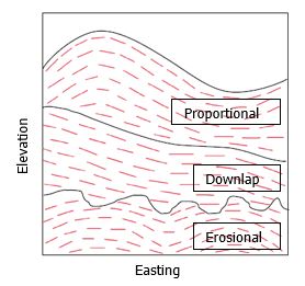
When the continuity of the variable of interest follows a known structural surface, the tangent of that surface can be used to infer the LVA field (Figure 8). This is usually well supported in software and the dip of a surface can be calculated with built in functions. This does not provide the magnitude of anisotropy, but that is typically kept constant within each domain. This gives rise to the idea of ‘dynamic anisotropy’ where the magnitude of LVA is typically constant; note that ‘dynamic anisotropy’ is just a restricted case of LVA modeling. It is important to note that when LVA follows easily modeled surfaces, stratigraphic coordinate transformations (Latifi & Boisvert, 2022) are preferred over dynamic anisotropy with the LVA field obtained from the surfaces. In general, if coordinate transformation such as vein straightening, stratigraphic flattening, or cylindrical/spherical/etc. can be applied, they will outperform LVA modeling because they directly model the features that control the LVA.

Point Data

The axial nature of orientation data makes estimation of the LVA field from point measurements difficult. ‘Axial’ refers to data where the direction of propagation is unknown or irrelevant. When considering LVA, a variogram in the 45° direction is considered the same as a variogram in the 45°+90° direction. 2D axial data can be processed by doubling the angles before their decomposition (Figure 9). The angle is doubled, the sin and cos are estimated in the domain, the angles are reconstructed, and finally divided by 2. This doubling trick makes it so that 180° is identical to 360° and accounts for the ‘wrapping’ at 360°/0°.

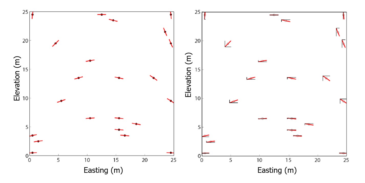
The doubling trick does not work in 3D, 3D axial data are defined by strike/dip/plunge or roll/pitch/yaw. These angles are converted into a quaternion representation (Lillah & Boisvert, 2015; Yang, 2012). Quaternion rotation is used to align the quaternions to a common reference frame, ensuring that they are in a consistent orientation before averaging (Figure 11). An average quaternion representing the average orientation is constructed by assigning weights to the quaternions and calculating their weighted average. The three quaternions are estimated exhaustively, similar to how the sin and cos values were estimated in 2D, then the quaternions are converted back into three angles (e.g., Euler angles) that exhaustively define the orientation of the LVA field.

Exhaustive Data

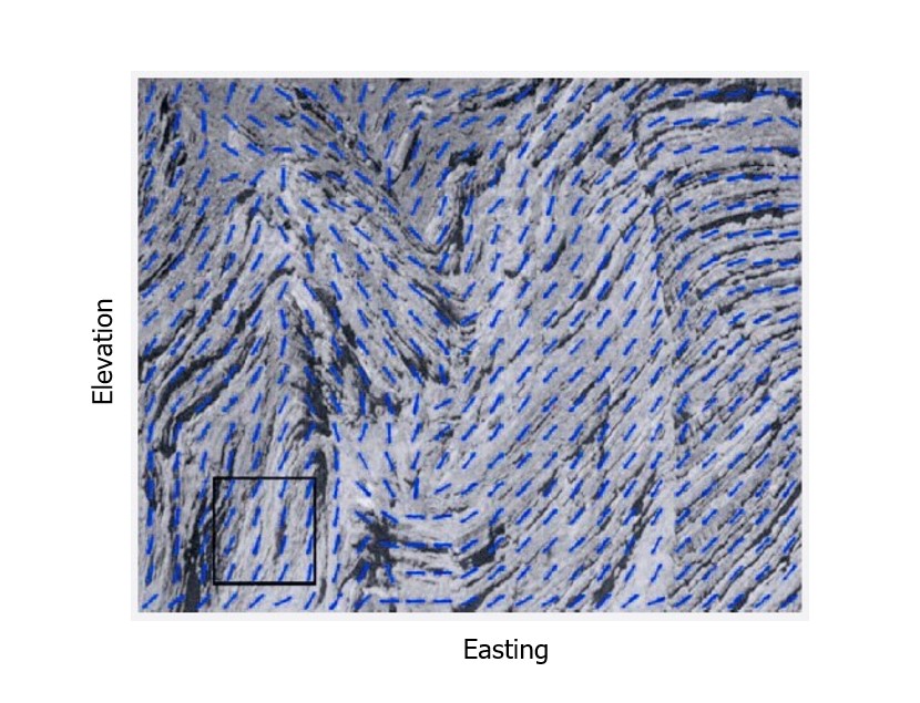
Often exhaustive secondary data, such as geophysical surveys, have the same local anisotropy features as the variable of interest. In these cases, the LVA field can be extracted from the exhaustive data and used in estimation or simulation. This is typically done with moving window methods where the LVA is inferred from local windows. One method is to calculate the gradient field g(\(u\)) for every point \(u\) from the exhaustive data (Lillah & Boisvert, 2012). Alternatively, the moment of inertia (Pyrcz & Deutsch, 2014) of the local window or its covariance map can be calculated and used to infer the local orientation of anisotropy (Lillah & Boisvert, 2012), as in Figure 10. It is difficult to infer a priori which moving window method will perform best for a given domain; the most common issue is that the angles are quite noisy and require smoothing after generating the LVA field, as the LVA field should be ‘smooth’; Think about modeling a trend in the mean (Harding & Deutsch, 2021) where the mean should vary smoothly in the domain, the same is true here for a trend in the anisotropy (a.k.a. LVA). It is recommended that multiple methods of LVA extraction be applied to the domain of interest and the modeller choose the one that is the most appropriate.

Summary

This lesson discusses the limitations of using fixed anisotropy in modeling geological domains and suggests locally modeling LVA to improve geostatistical models in complex geological settings. Three methods of incorporating LVA presented are 1) hard boundaries between domains, suitable for abrupt changes in anisotropy; 2) local variogram reorientation, assuming constant anisotropy within a defined search radius for smoothly varying anisotropy; and 3) modifying covariance between locations considering varying anisotropy within the search neighborhood, often using the shortest path distance (SPD) to account for curved continuity paths. Generating the LVA field is identified as a challenging step, with three approaches explored: 1) inferring LVA from known structural surfaces; 2) using doubling tricks or quaternion representations for processing axial data; and 3) extracting LVA from secondary data sources like geophysical surveys. LVA modeling is essential for capturing non-stationary anisotropies in complex geological settings, enabling improved representation of trends in the variogram.

References