Cite this lesson as: Dias, P.M., & Deutsch, C.V. (2022). The Decision of Stationarity. In J.L. Deutsch (Ed.), Geostatistics Lessons. Retrieved from http://www.geostatisticslessons.com/lessons/stationarity
The Decision of Stationarity
Paulo Mauricio Dias
University of Alberta
Clayton V. Deutsch
University of Alberta
June 8, 2022
Learning Objectives
- Review the concept of stationarity
- Evaluate the different types of stationarity
- Understand factors to be considered when deciding on stationarity
Introduction
Stationarity is an important concept in geostatistics. A decision of stationarity permits the statistical inference of probability. Most geostatistical applications consider the meaning of probability to be the proportion of times under similar circumstances. For example, a P10 to P90 interval for the resources implies that there is an 80% probability for the true resources to be within those bounds. The uncertainty in a global resource is accumulated from the uncertainty at many locations. The uncertainty at a location could be assessed through repetition. As a thought exercise, consider a coin of questionable lineage; the fairness could be ascertained by flipping it many times and observing the proportion of times heads or tails are seen. Some form of repetition is required to infer probability. The prediction at unsampled locations in a geological site is more complicated and repetition is secured through multiple data grouped together for common analysis.
Although every location is unique, multiple locations can be grouped together for statistical inference. The entire site of interest is divided into spatial domains or subsets that are considered one at a time. This is the first and most important aspect of stationarity. Secondly, within a spatial domain that belongs together based on geological considerations, there may be gradational variations. This is the second aspect of stationarity. Stationary cannot be checked directly from the data, yet is required for the development of geostatistics theory. The concept of a Random Function (RF) applied to a regionalized variable has proven itself in modeling geological phenomena. The statistical parameters that define an RF must be assembled by replication/repetition over a spatial domain since temporal repetition is not an option for geological variables.
This Lesson describes the concept of stationarity, different levels of rigor or restrictions on spatial distributions, and a review of practical considerations before making a final decision of stationarity.
Domain Selection
A reasonable definition of estimation domains has a crucial role in the reliability of resources and reserves. Choosing too-small domains leads to unreliable models because of complex domain boundaries and few data within the domains. Choosing too-large domains leads to unreliable models because different data and geological controls are mixed together. Estimation domains are based on geological and statistical considerations of the regionalized variables that are being predicted.

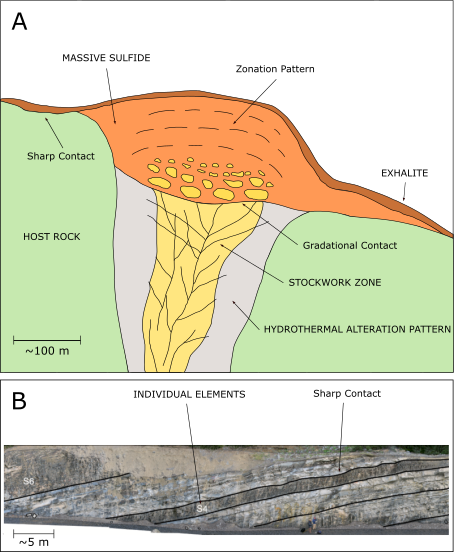
Figure 1-A presents an idealized VMS deposit type redrawn from (Lydon, 1984) with some geological features that can determine the continuity and disposition of an estimation domain. Formed by submarine vulcanism, VMS deposits usually show this schematic pattern with a hydrothermal alteration zone, a stockwork zone, and a massive sulfide zone. The stockwork zone presents a gradational contact with the massive sulfide zone and will determine grade continuity among both zones. The massive sulfide zone represents a region of lixiviation with a strong mineral zonation, making the grades vary from high to low grade. Defining estimation domains often requires the ability to understand the spatial behavior of these different zones and how other geological events changed the continuity of the grades.
Figure 1-B was modified from (Pyrcz & Deutsch, 2014) and presents an example of an outcrop considered an analog to some reservoirs. In general, reservoir facies constitute sediments accumulated along the channel meandering in which granulometry and thickness vary according to the depositional environment and their eroded source. It forms a series of intercalated sandstone and shale or mudstone-type rock layers. Note the presence of sharp contacts between these large-scale and fine-scale features. The importance of choosing the relevant layering and facies within the layers is evident. The continuous permeability and porosity properties will be controlled by this decision.
Statistical summaries are also used to help choose estimation domains. Ideally, the within-domain variability is small and the between-domain variability is large. Multivariate cluster analysis may help when considering multiple variables. Variograms may also be considered; the spatial continuity should be consistent within domains and potentially different between domains.
Once the domains have been defined at the data locations, a boundary model is needed to delimit the domains away from the data locations. Surfaces or 3-D closed volumes are established by different methods. The reliability of the boundary model depends on the amount, quality, and source of information available (McLennan, 2007). A traditional approach to determine geological boundaries is to define the interpreted limits on many horizontal and vertical sections, then connect them together into a 3-D model of the domains. Other implicit and geostatistical methods could also be used to create boundary models. All available information is considered including multiple drilling types, geological mapping and geophysical information.
There are other considerations in the definition of domain boundaries. In some cases, the domains are defined hierarchically with different controls at large scale versus small scale. Large scale domains are defined first, then subdivided. In other cases, post depositional folding, faulting or erosion must be considered.
Another essential aspect is that uncertainty in boundary position increases away from the data locations. It is particularly true when the scale of variability is less than the drill hole spacing. If the uncertainty is considerable, then a stochastic method may be considered to construct realizations of the boundaries. Additionally, when stochastically modeling domains within large areas, we ought to consider separate decisions of stationarity among them.
Stationarity
The first aspect of stationarity is the choice of domains within which to perform geostatistical calculations. Abrupt changes in the regionalized variable are often captured in the domain definition. The second aspect of stationarity is the location dependence of statistics within the domain. There is no access to all details of the complex geological processes that led to our deposit; we observe the result and make reasoned judgements about the location dependence of statistical parameters. A stationary process is one where the unconditional joint probability distribution does not change when shifted in time or space.
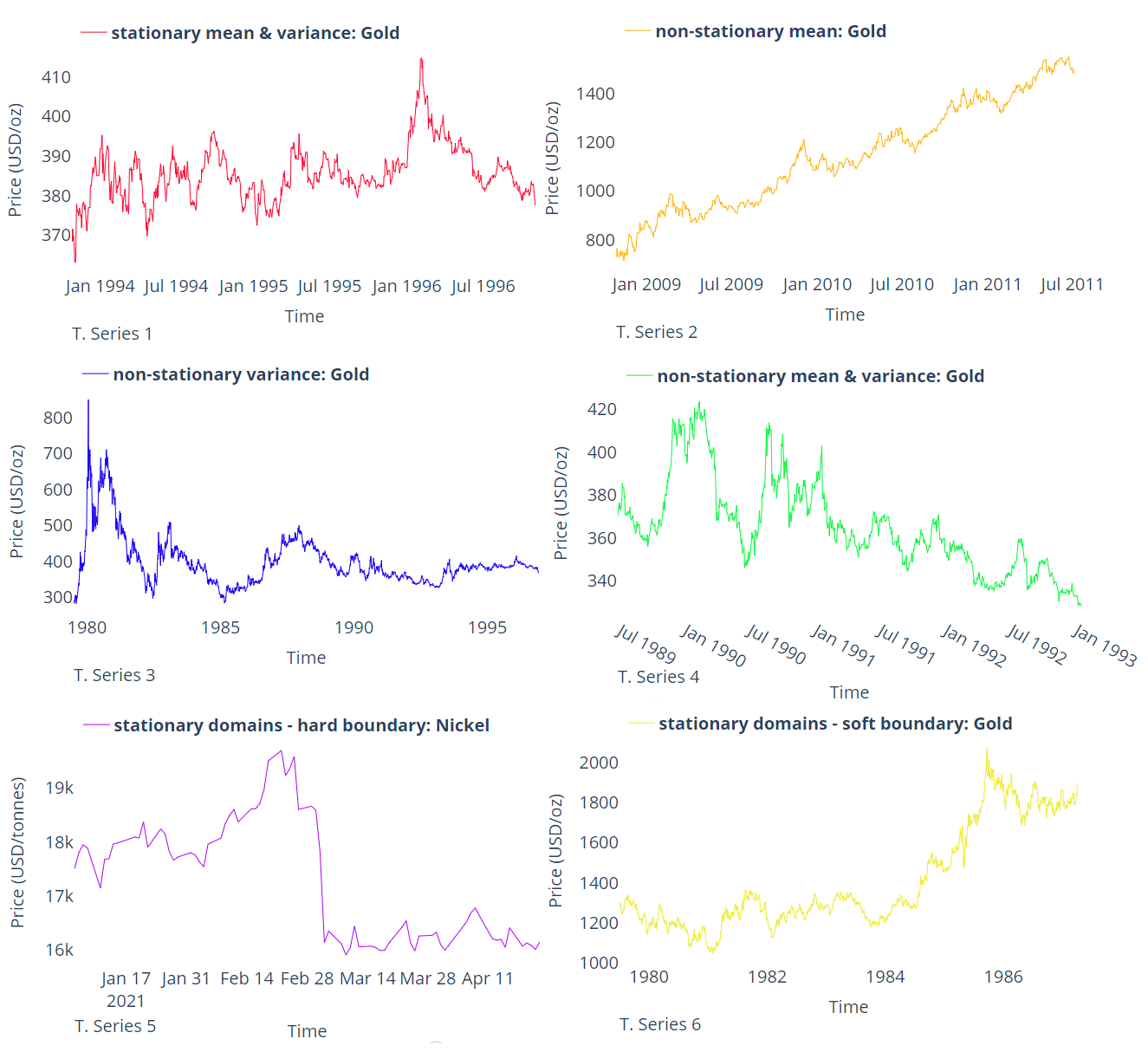
A time series is a family of random variables defined on a probability space in which a covariance function expresses the dependence between them (Brockwell & Davis, 1991). A time series is said to be stationary if it has a finite variance, a constant mean, and the autocovariance function dependent only on the lag vector for a given time interval. Figure 2 presents six different examples of time series and their stationarity behavior.

More generally, a stochastic process is said to be stationarity if all n-dimensional distributions are independent of the period (Lindgren, 2012). A random function (RF) is defined as a set of random variables (RV) over a domain \(A\). If we assume a certain level of homogeneity of the statistical parameters over \(A\), we can say that the experimental values (samples) represent a realization of the same RF over all the domain \(A\). This permits inference of the parameters of the RF. Different stationarity types are defined according to the level of homogeneity. If all moments and the multivariate distributions of the RF are invariant under translation, the RF is said to be strict-stationary or strong-stationary:
\[F(\mathbf{u}_{1}, ...,\mathbf{u}_{k} ; z_{1}, ..., z_{K}) = F(\mathbf{u}_{1} + \mathbf{h}, ..., \mathbf{u}_{k} + \mathbf{h}; z_{1}, ..., z_{K}) \:\:\:\:\:\:\:\:\:\: \forall \:\: \mathbf{h} \in A\] Where \(\mathbf{u}\) is a coordinate vector, \(\mathbf{h}\) is a separation vector between two locations, also refered as lag vector.
Strict stationarity is the most restrictive case. Most mining and petroleum applications do not require that all distributions of the RF \(Z(\mathbf{u})\) be invariant under translation. If the first moment, the mean, is invariant under translation the RF is said to be first-order stationarity. If the first two moments are considered invariant under translation, the RF is considered to be second-order stationarity. First and second order stationarity are sometimes referred to as weak stationary or wide-sense stationary. In this case, the covariance will exist if the variance is finite (David, 1979). The two moments of a RF are defined as:
- Expected Value
\[E\{Z(\mathbf{u})\} = m, \:\:\:\:\:\:\:\:\:\: \forall \:\: \mathbf{u} \in A\]
- Variance
\[C(0) = E\{[Z(\mathbf{u}) -m]^{2}\} = \sigma^{2}, \:\:\:\:\:\:\:\:\:\: \forall \:\: \mathbf{u} \in A\]
- Covariance
\[C(\mathbf{h}) = E\{Z(\mathbf{u} + \mathbf{h}) \cdot Z(\mathbf{u})\} - [E\{Z(\mathbf{u})\}]^{2}, \:\:\:\:\:\:\:\:\:\: \forall \:\: \mathbf{u}, \mathbf{u} + \mathbf{h} \in A\]
- Variogram
\[2{\gamma}(\mathbf{h}) = Var\{Z(\mathbf{u} + \mathbf{h}) -Z(\mathbf{u})\}, \:\:\:\:\:\:\:\:\:\: \forall \:\: \mathbf{u}, \mathbf{u} + \mathbf{h} \in A\]
A stationary random function (SRF) commonly refers to second-order stationarity. It is also the most common decision when working with Simple Kriging. When this assumption is limited for any practical reason to only the variance of the increments of two variables separated by a lag vector \(\mathbf{h}\) (the variogram), the RF is then said to have intrinsic stationarity. This is valid when there is a significant trend, see (Journel & Huijbregts, 1978) and (Krige, 1982). The second-order stationarity assumption is also equivalent to IRF-0 (intrinsic random function of order zero), which lies among the IRF-k generalization. The idea is to create increments of sufficiently higher orders to reach stationarity for those cases where the regionalized variable itself is not stationary (Chilès & Delfiner, 2009).
Quite often, due to the nature of the geological phenomenon, the assumption of stationarity is limited to a spatial extension \(b\), usually representing a volume from which samples are retained in a local search (\(\vert\mathbf{h}\vert \le b\)). In this situation, the RF is said to be quasi stationary or local stationary and is valid for the two previously mentioned cases. It is the most common decision taken when applying Ordinary Kriging and locally varying anisotropy (LVA) in the variogram within search neighborhoods.
The concept of an RF allows consideration of many variables \(K\) simultaneously. The inference of the one-point and two-point moments require an assumption of joint stationarity (Goovaerts, 1997). The different cases related to stationarity, such as strict, second-order, intrinsic, and quasi are applied to the multivariate case. Figure 3 summarizes the stationarity types relating to a level of homogeneity.

The decision of stationarity depends mainly on the level of statistical homogeneity observed. Ordinary Kriging is by construction limiting the stationarity to a given neighborhood - quasi-stationary. Simple Kriging assumes strong stationarity. The Gaussian related techniques like multiGaussian kriging and most simulation also assume strict stationarity. Categorical variables are almost always non stationary and simulated with a modeled trend in the proportions. In the presence of a trend, when the first-order moment varies over the domain, making it non-stationary, it must be removed and the remaining residuals treated as stationary (Harding & Deutsch, 2021). A simple residual is rarely considered in modern applications. A stepwise conditional transform of the variable considering the trend accounts for complexities and constraints.
Discussion
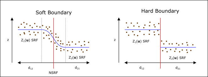
After defining the estimation domains, the nature of the contacts between domains is assessed to see if they are gradational (soft) or sharp (hard), as presented in Figure 4, modified from (McLennan, 2007). The grades in proximity to the contact are plotted and evaluated to understand the nature of the contacts; an abrupt change of grades on both sides of the contact implies a hard contact; see time series 5 in figure 2. On the contrary, similar grades on both sides of a contact may imply a soft contact; see time series 6 in figure 2. The covariance across the domain boundaries may also be investigated; a significant covariance may imply a soft contact. There are different ways to account for soft contacts. The simplest approach is to share data across the contact. A model of corregionalization could be used to implement cokriging with data from multiple domains. As another alternative, a mixing model could be adopted to account for these transitional zones (Larrondo & Deutsch, 2005).

Additionally, the decision of stationarity within domains must consider the possible presence of trends. A trend is a large-scale tendency of a geological phenomenon and is considered deterministic. A trend implies at least non-stationarity of the first moment \(m(\mathbf{u})\) over the domain. The trend can be visually identified and supported by geological evidence, such as mineral zoning. A modern approach to building a trend model and modeling in presence of the trend is summarized in (Harding & Deutsch, 2021).
The decision of stationarity also applies to multi-point geostatistics. This method considers more than two-point statistics at the same time. The frequencies of patterns of the RF are inferred by scanning a training image using a multiple-point pattern without regard for its location. The multiple point statistics are considered to be stationary in most applications (Strebelle & Zhang, 2005). Some alternatives for applying MPS for non-stationary are patter-base and location-based methods (Yin & Feng, 2017).
Summary
Stationarity is a crucial concept underlying geostatistical-related methods for numerical geological modeling. Understanding the conceptual geological model relevant for a site is important. The depositional and diagenetic alteration processes would create volumes of rock that should be kept together for common analysis. Once the domains are defined, the details of contacts and trends will define the type of stationarity employed in subsequent estimation and simulation.