Learning Objectives

• Review the concepts of stationarity
• Appreciate trend modeling and modeling with a trend
• Demonstrate the importance of trend modeling in modern geostatistical workflows
• Understand the techniques and checks implemented (source code available).

Introduction

A trend is a large-scale prevailing tendency or pattern related to an underlying geologic phenomenon. Trends are common in natural processes, such as a fining-upward sequence in a reservoir sandstone or a decrease in metal grades away from a porphyry intrusion. In the context of geostatistics, a random variable is commonly represented by its decomposition into a smooth deterministic trend component and a stochastic residual (Chilès & Delfiner, 2011). The trend represents the behaviour of the geologic process at a large scale, while the residuals represent the local short-scale variability.

An implicit assumption of geostatistical prediction algorithms is “stationarity”, that is, the spatial statistics of the random variable are invariant to the location within the domain (Isaaks & Srivastava, 1989). The presence of large-scale trends violates this assumption of stationarity as the mean is location-dependent. The goal of modeling with a trend is to remove the large-scale deterministic trend component from the random variable to satisfy the assumption of stationarity (Qu, 2018). Simulation or estimation can then proceed with the deemed-stationary residuals.

Stationarity

The decision of stationarity groups or pools relevant data together. As data replicates are not available at location \(\mathbf{u}\) to infer the random function \(Z(\mathbf{u})\), geologically similar data must be pooled such that population statistics can be reliably inferred. This decision of stationarity allows the trade of unavailable replicates at the same location for data at other locations to infer the mean, variance and covariances (Deutsch & Journel, 1998). Pooling too little data may lead to unreliable statistics, and too many data may lead to masking of important geological features. Stationarity is a property related to the underlying random function model and cannot be checked or validated with data (Goovaerts, 1997).

Inference of the first and second order moments (mean and covariance) of the random function are required for geostatistical estimation algorithms. When divided into a sub-region \(A\), the variable of interest is considered first-order stationary if the expected value is constant within \(A\). The variable is second-order stationary if the covariance depends only on the separation vector \(\mathbf{h}\) within \(A\). A random function \(Z(\mathbf{u})\) is second-order stationary when:

\[ E\{Z(\mathbf{u})\} = m \] \[ E\{Z(\mathbf{u}) - m^2\} = C(0) = \sigma^2 \] \[ E\{Z(\mathbf{u}) \cdot Z(\mathbf{u} + \mathbf{h})\} - m^2 = C(\mathbf{u}, \mathbf{u}+\mathbf{h}) = C(\mathbf{h}) \] \[ \forall \ \mathbf{u}, \mathbf{u}+\mathbf{h} \in A \]

Where \(m\), \(\sigma^2\) and \(C(\mathbf{h})\) are the mean, variance and covariance, respectively, and do not depend on location. The invariance of the random function parameters to location within \(A\) allows the relation \(C(\mathbf{h}) = \sigma^2 - \gamma(\mathbf{h})\) where \(\gamma(\mathbf{h})\) is the (semi)variogram model. This is the foundation of variogram interpretation (Pyrcz & Deutsch, 2014).

Trends

Geologic variables typically exhibit trends that can be explained by the depositional and diagenetic processes. Trends are smooth gradual large-scale changes in the expected value of both continuous and categorical variables. Trends can be detected through prior geologic understanding or by visualizing contour maps, interpreted models or moving window averages across the region. Experimental variogram points that rise above the sill may also indicate the presence of a trend.

The spatial distribution of geologic variable in the presence of a trend can be decomposed into a deterministic and a random component (Wackernagel, 2003):

\[ Z(\mathbf{u}) = m(\mathbf{u}) + R(\mathbf{u}) \ \ \ \forall \ \mathbf{u} \ \in A\] \[ E\{R(\mathbf{u})\} = 0 \] \[ E\{Z(\mathbf{u})\} = m(\mathbf{u}) \]

Where \(m(\mathbf{u})\) is the deterministic location-dependent mean and the random variable \(R(\mathbf{u})\) is the spatially correlated residual. The correlation between the mean and the residual is assumed to be zero, \(\rho \{m(\mathbf{u}), R(\mathbf{u})\} \approx 0\) (Qu, 2018). This is not always the case due to most geologic variables being positively skewed. This locally varying mean violates the assumption of first-order stationarity and should be explicitly accounted for before geostatistical modeling (McLennan, 2007).

Trend Modeling

The goal of trend modeling is to model the smooth large-scale deterministic component of the regionalized variable. Trend models are built using the available data, which leads to a degree of subjectivity. Trend features appear different at different scales. The modeler must choose the level of variability represented by the trend. Neither over-fitting nor under-fitting the trend is desirable. Over-fitting the deterministic component can result in too little variability in the residuals. Over-fitting leads to too little variability in the final geostatistical model (Pyrcz & Deutsch, 2014). Under-fitting may lead to models that do not reproduce the observed geologic trend. Human intuition is reasonably good at detecting over- or under-fitting. McLennan (2007) suggests that the variability accounted for by the trend should be no more than 50% of the data variability, although this is also subjective. There is no objective measure of trend “goodness.” Rationality checks include if the mean of the trend model matches the declustered mean of the data that is equivalent to the mean of the residuals being equal to zero.

There is a wide range of methods to generate trend models. Common approaches in geostatistics include kriging (Deutsch & Journel, 1998) and moving window averages (Manchuk & Deutsch, 2011). Kriging is a practical tool to build trend models with the correct parameters. The search, variogram model and block discretization are important considerations. A trend model must be smooth. Search artifacts when using a restricted search is a known issue with kriging. A smooth map can be generated using a large search or global kriging if the number of data permits. The variogram model for kriging the trend is constructed separately from the variogram of the underlying variable. The trend variogram model should have a large nugget effect (30-40%) while the range controls how quickly the trend approaches the global mean away from the data. Block kriging should be employed to ensure the trend model does not reproduce the data exactly.

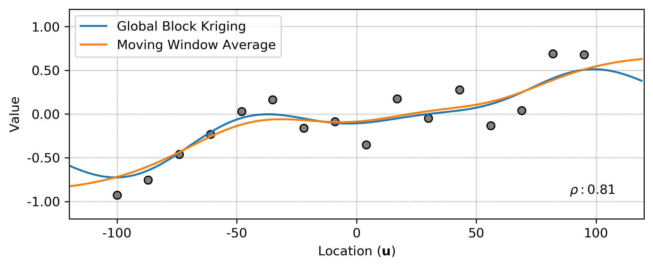
Moving window averages are a simple approach to fit a trend to observed data. A window is centered on an unsampled location, \(\mathbf{u}\), and the weighted average of the samples within each window is assigned to the location:

\[m^*(\mathbf{u}) = \frac{ \sum_{i=1}^n w_i \cdot z(\mathbf{u}_{i}) }{ \sum_{i=1}^n w_i } \ \ \ \forall \ \mathbf{u} \ \in A\]

Where \(z(\mathbf{u}_{i})\) is a sample at location \((\mathbf{u}_{i})\), \(w_i\) are weights and \(n\) is the number of samples within the window. Any window geometry, averaging process and spatial weighting function within the window are valid. Equal weighting amounts to the arithmetic average. Distance weighting is common within geostatistics, where closer data receive greater weight. Gaussian-like weighting functions (Manchuk & Deutsch, 2011; Qu, 2018) generate spatial weights that gradually decrease from the window center and prevent discontinuities or artifacts. The window size is an important consideration as it controls the amount of variability imparted in the trend. A very small window leads to data reproduction and maximum variability, while a very large window leads to an under-fit trend with little variance. In contrast to kriging where the screening effect can lead to negative weights, a moving window average will never exceed the data values.

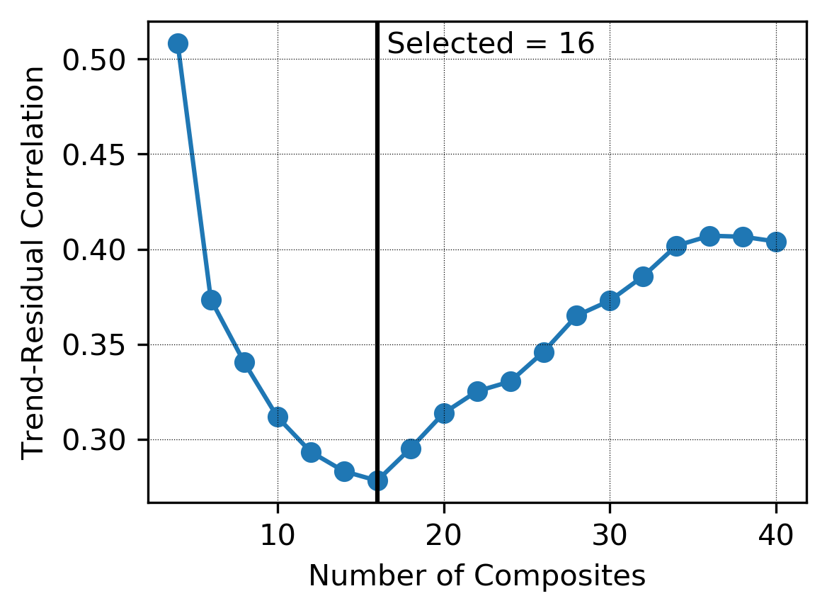
Consideration must be given to the search/window anisotropy and the number of neighbouring data to consider. The anisotropy of the search window should be less than the anisotropy of the underlying variable. A general starting point is the square root of the anisotropy ratio of the observed data, \(A_{trend} \approx \sqrt{\frac{a_{hmax}}{a_{hmin}}}\). Both window size and the number of data affect the smoothness of the trend and, ultimately, the proportion of total variance it describes. There are no objective rules for window size; however, it should be large enough to average sparsely sampled regions but small enough to not under-fit. One approach for selecting the maximum number of data to retain is considering the correlation between the residuals and the resulting trend model (Qu, 2018). One could select the number of composites that minimizes this correlation before applying a scaling factor to further smooth the trend. Case studies suggest that a scale factor of 1.8-2.0 times the number of composites that minimize the correlation is reasonable (Qu, 2018). This criteria is highly dependent on the number of available data and in practice may be hundreds of composites. A minimum of 100-200 composites is typically used in practice for all but extremely sparse or 2D data sets.

Though these recommendations may provide a reasonable starting point, they are not definitive, and the practitioner should exercise judgment over the resulting trend model. The visual texture, cross validation studies, and resulting variograms should be assessed when evaluating a trend model.

Traditional Approach to Modeling with a Trend

The traditional approach to modeling with a trend is to subtract the collocated trend values from the observed data \(z(\mathbf{u}_i)\) to obtain residuals, perform estimation or simulation with the residuals, and then add back the trend values (Isaaks & Srivastava, 1989). The workflow is summarized as:

1. Model the exhaustive trend \(m^*(\mathbf{u}) \ \ \forall \ \mathbf{u} \ \in A\)
2. Calculate the residuals using the collocated data-trend values as \(r(\mathbf{u}_i) = z(\mathbf{u}_i) - m^*(\mathbf{u}_i)\)
3. Calculate and model the variogram of \(r(\mathbf{u}_i)\)
4. Perform estimation or simulation with \(r(\mathbf{u}_i)\)
5. Calculate the final estimate as \(z^*(\mathbf{u}) = m^*(\mathbf{u}) + r^*(\mathbf{u}) \ \ \forall \ \mathbf{u} \ \in A\)

This approach can work well if the trend does not explain a significant proportion of the variance and \(r(\mathbf{u}_i)\) and \(m^*(\mathbf{u}_i)\) are nearly independent. The main drawback of this approach is the constrained bivariate trend-residual relation imposed by the decomposition of a strictly non-negative random variable, \(Z(\mathbf{u})\).

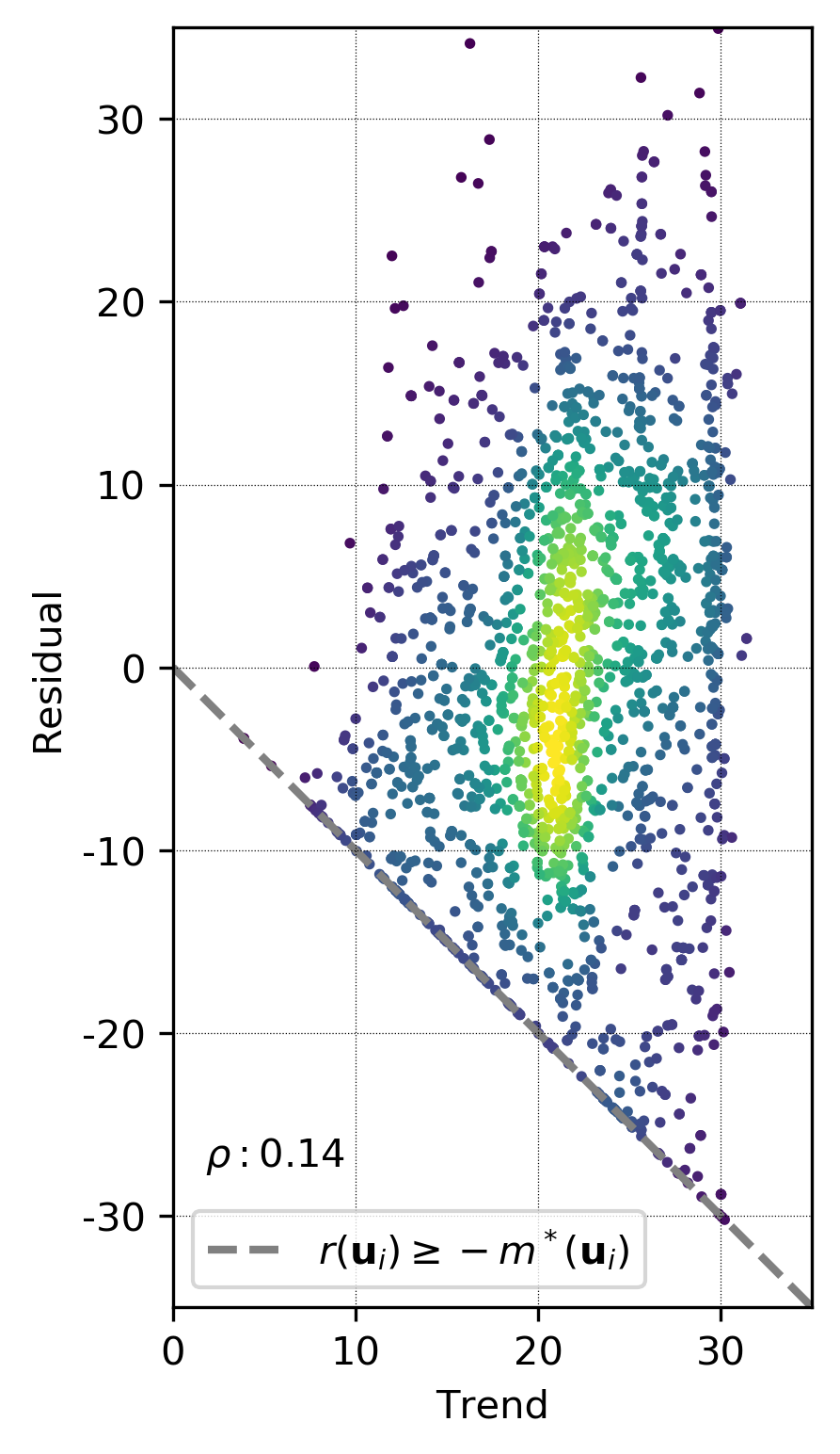
To ensure non-negative values of \(Z(\mathbf{u})\) when the trend is added back, simulated residuals must honor the relationship \(r^*(\mathbf{u}) \geq -m^*(\mathbf{u})\). This must be handled explicitly. Geostatistical simulation algorithms provide no control for reproducing this constraint and the addition of residuals and the trend component does not ensure positivity at all locations (Leuangthong & Deutsch, 2004).

Modern Approach to Modeling with a Trend

The modern approach to modeling with a trend is to perform a stepwise conditional transform (SCT) (Leuangthong & Deutsch, 2004) of the observed data \(z(\mathbf{u}_i)\), given the deterministic trend component \(m^*(\mathbf{u}_i)\). The conditional distributions required for the SCT are calculated from a Gaussian Mixture Model (GMM) fitted to the collocated data-trend values (Qu & Deutsch, 2018). The use of a GMM removes the possibility of binning artifacts during the SCT. This is aimed at probabilistic modeling and not estimation. Estimation would proceed in a similar fashion to the traditional workflow. The probabilistic workflow is summarized as:

1. Determine the representative distribution \(F_z(z)\)
2. Normal score transform the data as \(y_{z_i} = G^{-1}(F_z(z_i)), \ \ i=1,...,n\) using declustering weights
3. Model the exhaustive trend of the normal scores as \(y_m^*(\mathbf{u}) \ \ \forall \ \mathbf{u} \ \in A\)
4. Normal score transform the trend model as \(y_{m_i} = G^{-1}(F_m(m_i)), \ \ i=1,...,N\)
5. Fit a GMM to the collocated results of steps 2 and 4 using declustering weights
6. SCT of the normal score data conditional to the trend using the fitted GMM from step 5 \(y^{\prime}_{z_i} = G^{-1}(F_{z|m}(y_{z_i}|y_{m_i})), \ \ i=1,...,n\)
7. Calculate and model the variogram of \(y^{\prime}_{z_i}\)
8. Simulate \(y^{\prime}(\mathbf{u}) \ \ \forall \ \mathbf{u} \ \in A\)
9. Reverse the GMM-SCT and then reverse the normal score transform to obtain \(\{z^l(\mathbf{u}) \ \ \forall \ \mathbf{u} \ \in A, \ \ l=1,...,L\}\)

Where \(n\) is the number of data, \(N\) is the number of grid nodes and \(L\) is the number of realizations. Transforming both the data and the trend model to be marginally standard normal improves the fitting of the GMM (Silva & Deutsch, 2016). The transformation of the data values conditional to the trend explicitly removes all trend-like features from the data and results in residuals that are uncorrelated with the normal score trend at lag \(\mathbf{h}=0\).

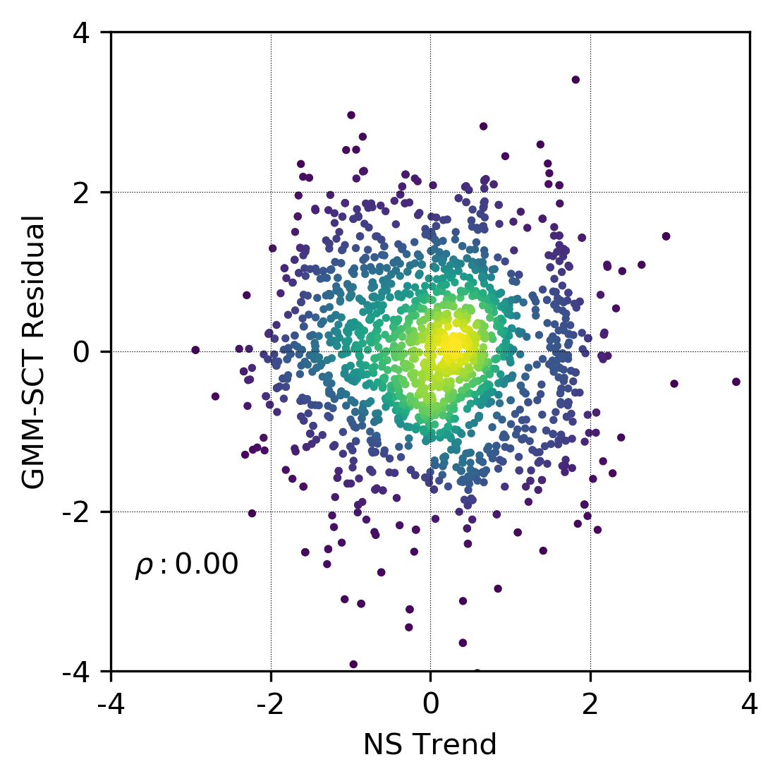
Unlike the traditional approach, the GMM-SCT procedure ensures the bivariate residual-trend relationship is reproduced and no negative values are simulated.

Simulation with a Trend Example

The following sections discuss steps 3-9 of the modern approach utilizing a clustered two-dimensional data set. The details of cell declustering and the normal score transform are presented in standalone lessons. Declustering and normal score transformation are necessary prerequisite steps to the trend modeling and modeling with a trend workflow.

Trend Identification

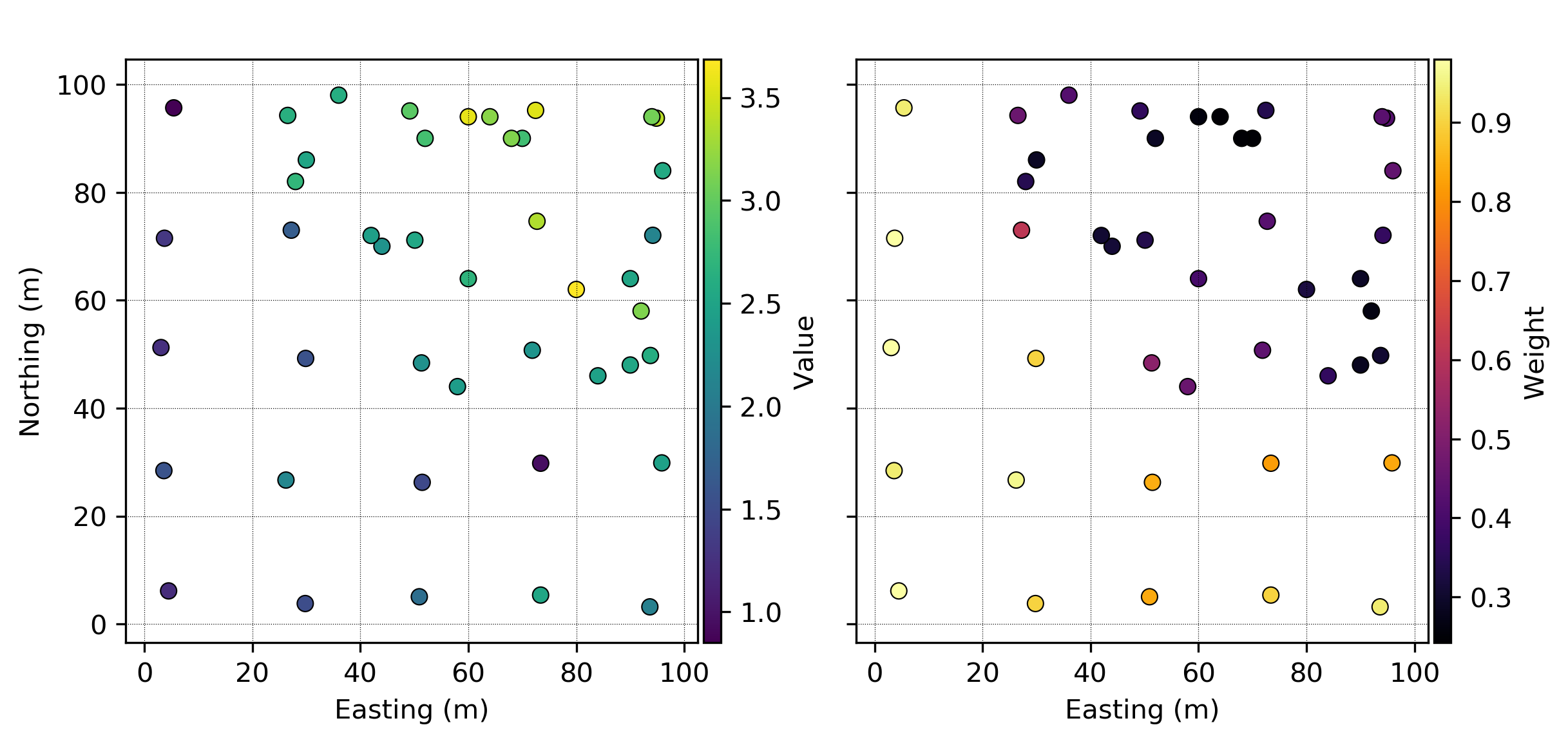
The presence of a trend may be identified visually; in the location plot of the data values, there is a gradual change from low values in the southwest corner to higher values in the northeast corner. The presence of a trend can also be identified through variography.

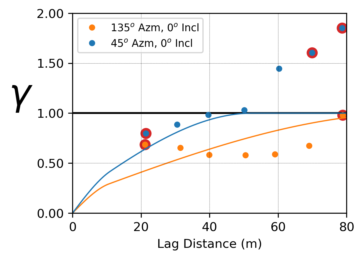
In this example, the experimental variogram of the normal scores continues to rise above the sill in the minor direction (045 degrees) as the lag distances increases. The variogram rising above the total variance suggests the presence of a trend in that direction.

Trend Modeling

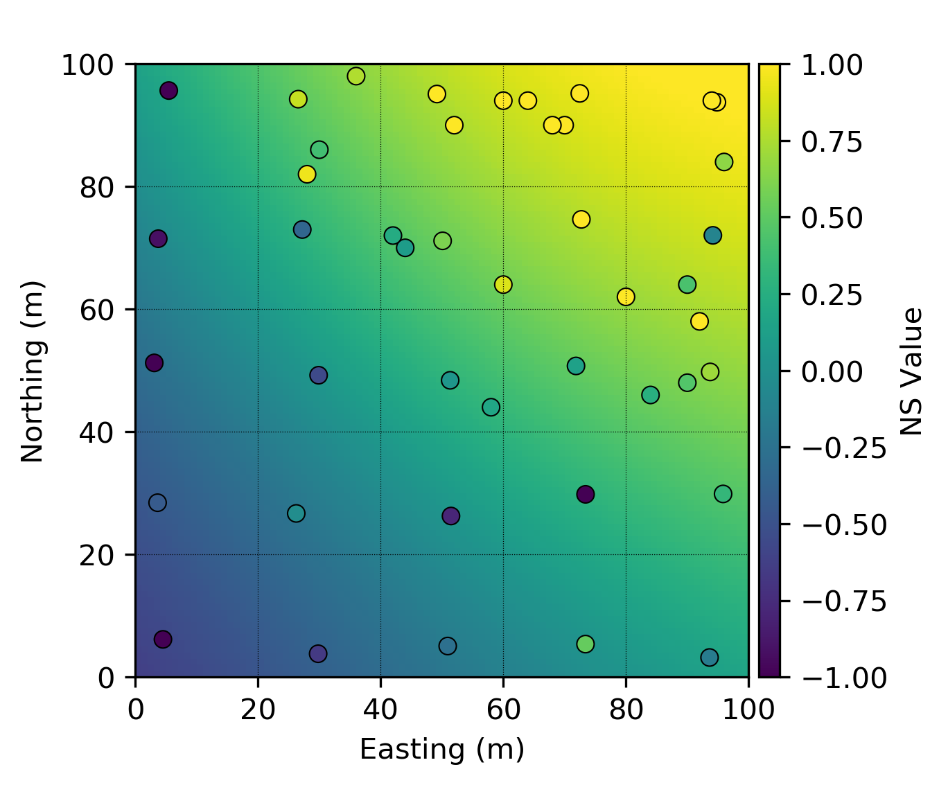
The first step in trend modeling is to determine an algorithm and spatial weighting function for trend construction. This example uses a moving window average with a Gaussian weighting kernel. The trend model is calculated using all available data with an anisotropic kernel window oriented in the direction of greatest continuity at 135 degrees. Note how the trend model shows smooth large-scale variation and does not exactly reproduce the data.

Gaussian Mixture Model

The exhaustive trend model of the normal scores is normal score transformed to standard normal, \(N(0,1)\). No declustering weights are necessary for the transform as the trend model is exhaustive. Collocated data-trend values are extracted for GMM fitting. The number of kernels to fit must be chosen. Visual inspection of the bivariate data-trend scatter plot can indicate complexity. The fewest number of kernels that still adequately capture the bivariate complexity should be chosen. Practically this number is between 2-5. Declustering weights should be considered in GMM fitting.

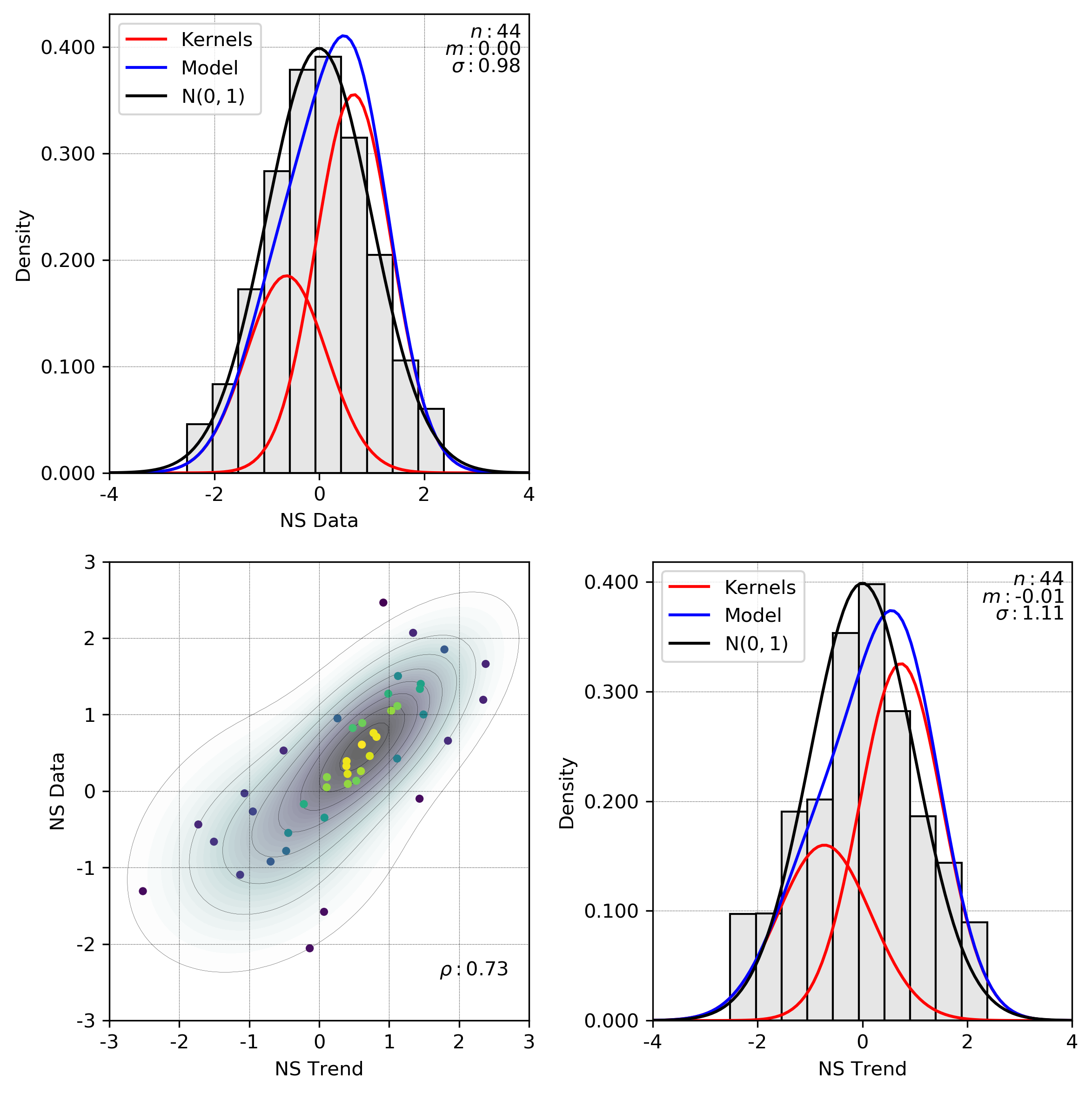
The GMM is fit with two kernels. The bivariate data-trend scatter (bottom left) does not show complex relationships though this could be a result of few data. The red curves overlaid on the univariate distributions are the Gaussian kernels, and the shaded contours in the scatter plot represent the multivariate probability density modeled by the GMM. The marginal distributions from the GMM are not perfectly normal; however, the deviation appears reasonable given the number of data.

Stepwise Conditional Transform

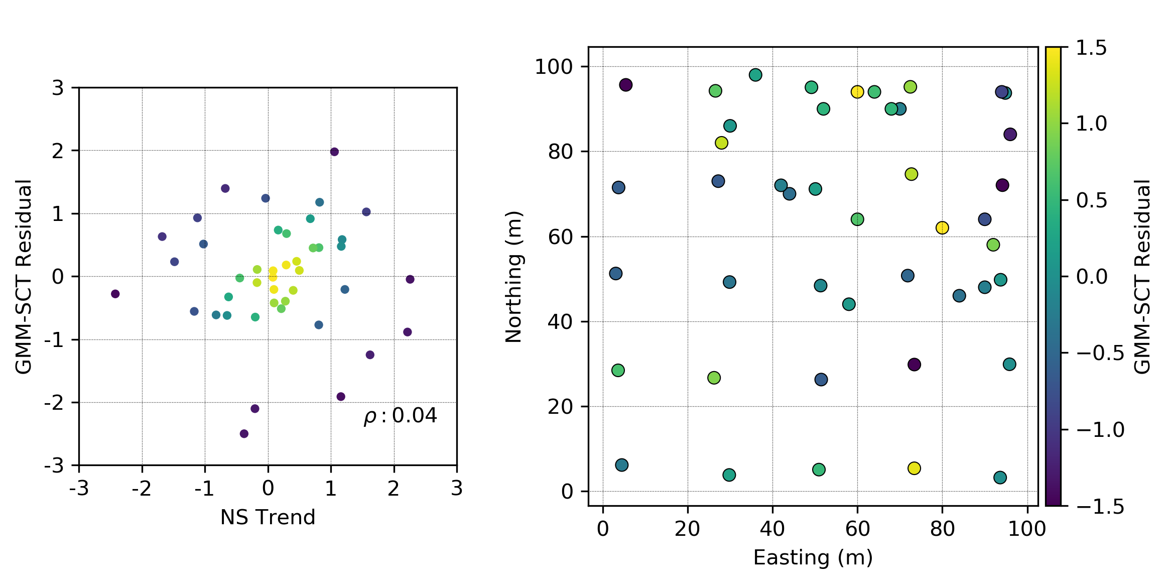
The normal score data is then transformed conditional to the collocated trend component using the fitted GMM. The resulting residuals are uncorrelated with the normal score trend. The large-scale trend component is not visually apparent in the location plot of the residuals.

Residual Variography

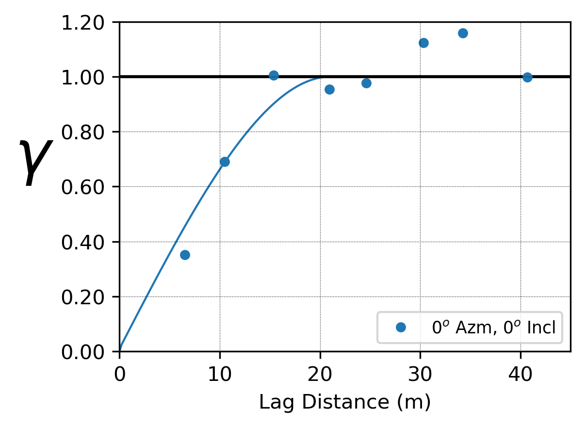
A variogram model of the residuals is required for simulation. A single structure omni-directional variogram model is fit to the experimental points. The fit of the trend model influences the resulting variogram structures. Some destructuring of the original variogram model is expected as long range continuity is embedded in the trend, but it should not be excessive. An over-fit trend model may lead to significant destructuring. The residuals should retain some spatial structure to be modeled, and the experimental variogram should not be pure nugget. If \(\gamma_R\) is pure nugget, the trend model is likely over-fit or modeling with a trend may not be necessary. That said, there is relatively little structure that remains in this example, despite a clear trend that is smoothly fit according to best-practice. In fitting the variogram model, consider that

• The nugget is not expected to be impacted by removal of a trend that captures only broad scale features, allowing for the modeled nugget to be selected with consideration of the normal scores nugget
• The trend is modeled with a muted version of the underlying anisotropy, so that the residual variogram is expected to maintain the same major/minor directions with reduced (but not inverted) anisotropy

These considerations are reflected in the displayed variogram fit.

Simulation

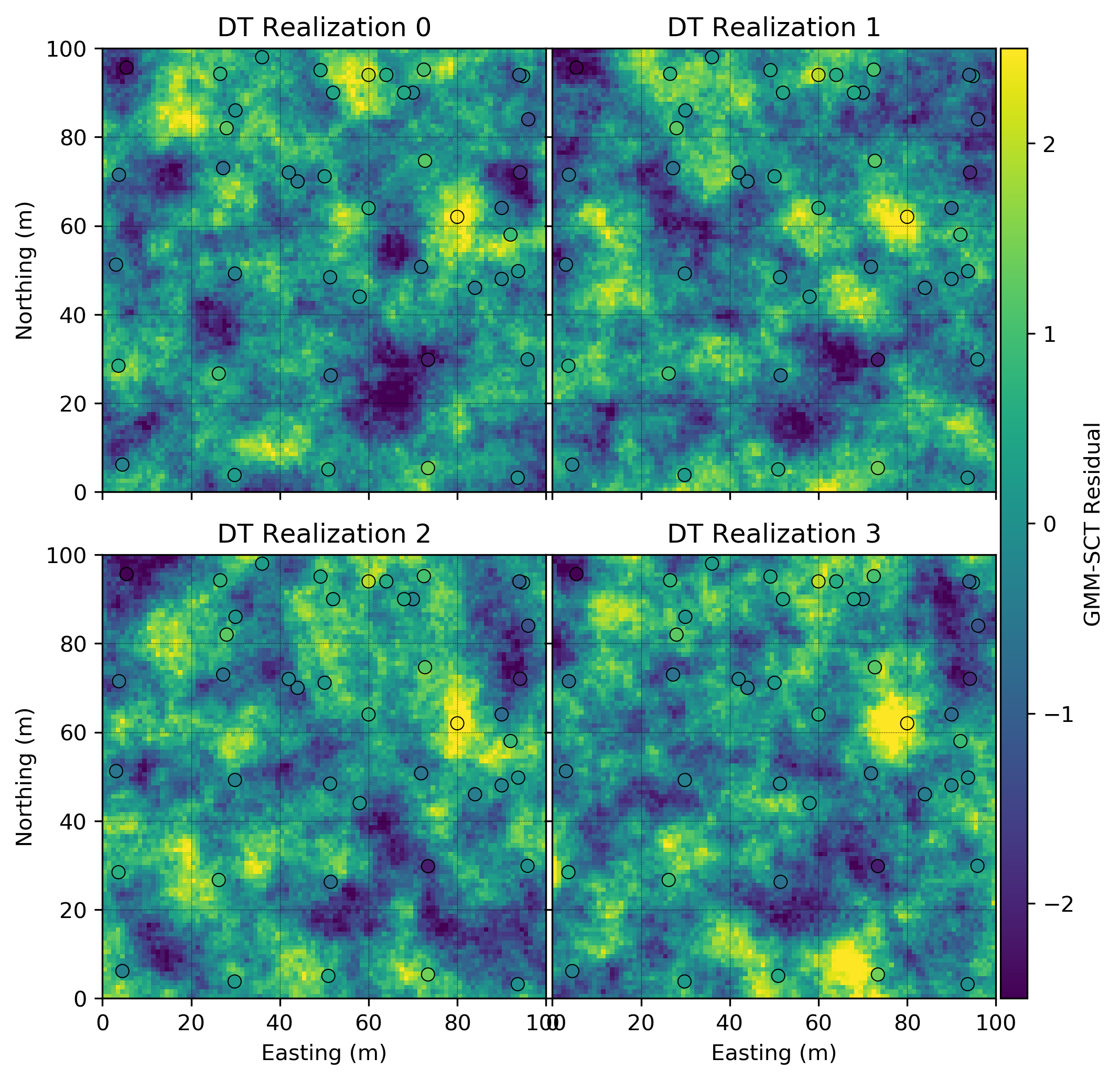
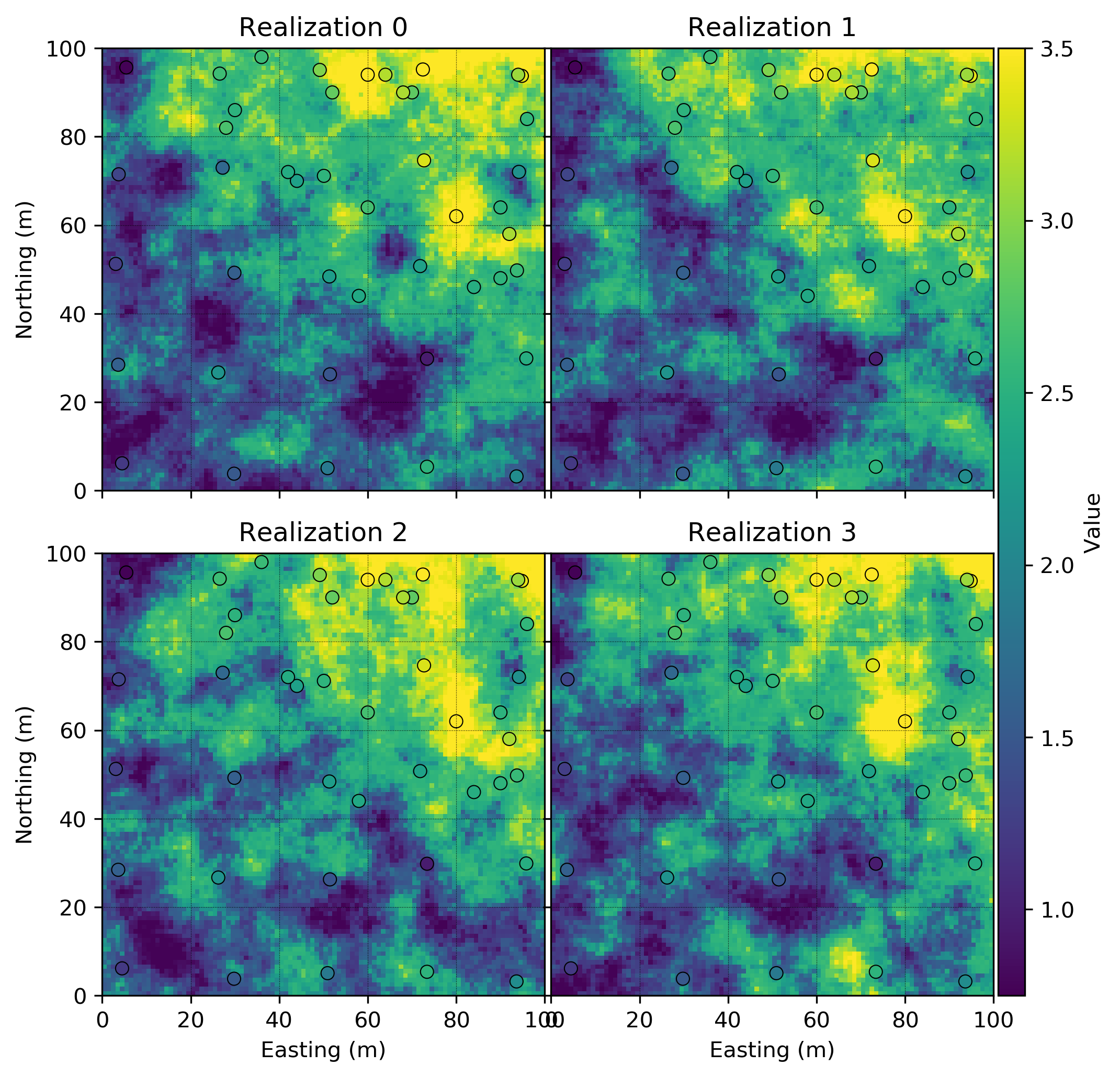
Simulation proceeds with the deemed-stationary residuals. This examples utilizes turning bands to simulate unconditional realizations which are then conditioned by kriging. The first four realizations are shown below. Note the lack of any trend-like features in the simulated realizations.

Back Transforms

The first back transform is the stepwise conditional back transform. The simulated residuals are transformed conditionally to the trend, reintroducing the trend component in normal score units. The first four realizations in normal score units are shown below.

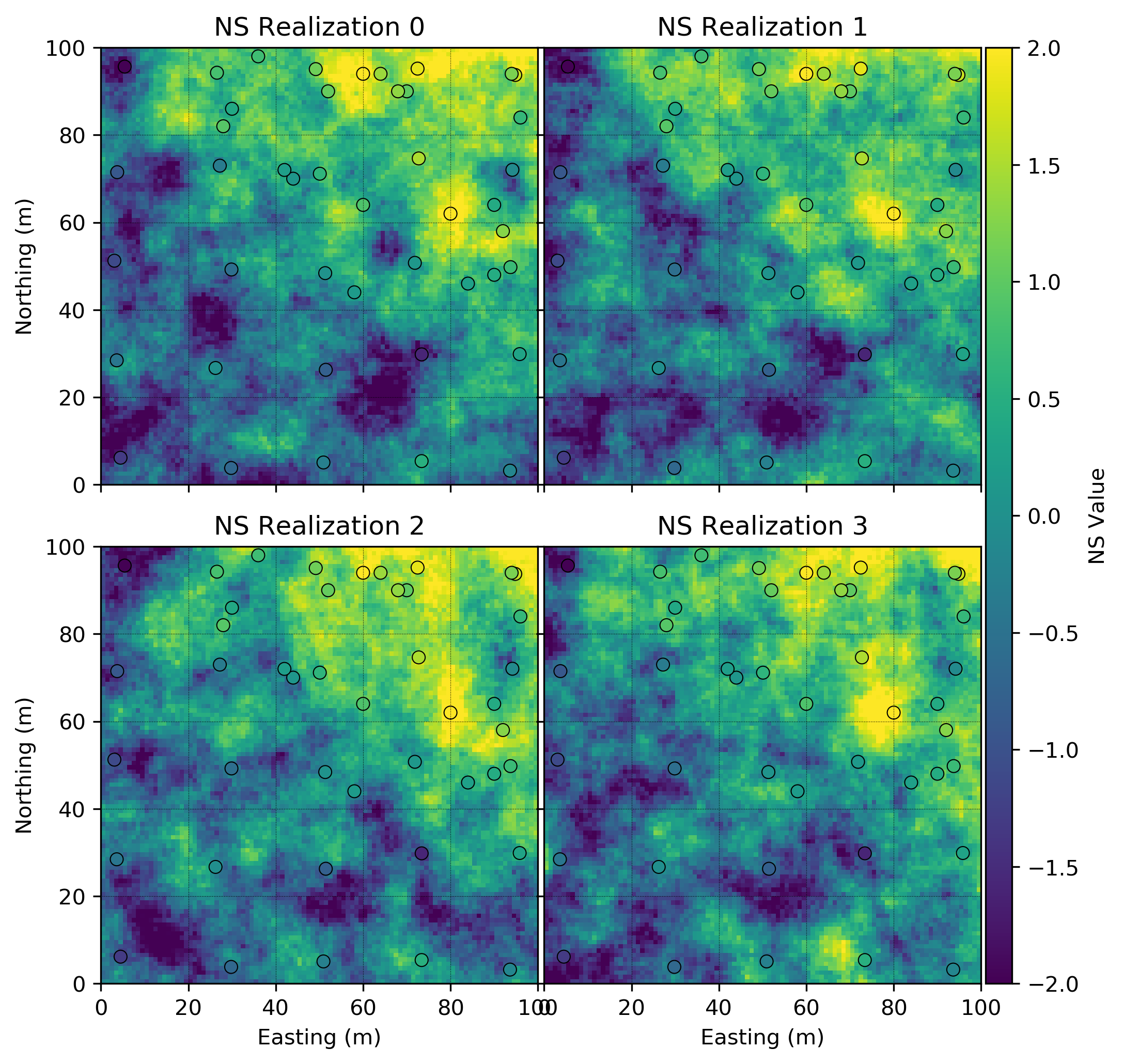
The second back transform is the normal score back transform. Gaussian units are back-transformed to original units. The first four realizations in original units are shown below. Note the presence of the NE-SW trend feature that has been reintroduced in the final simulated realizations.

Checking

Histogram reproduction is checked in original units, and variogram reproduction in normal score units. Variogram reproduction shows a trend in the minor direction which is expected.

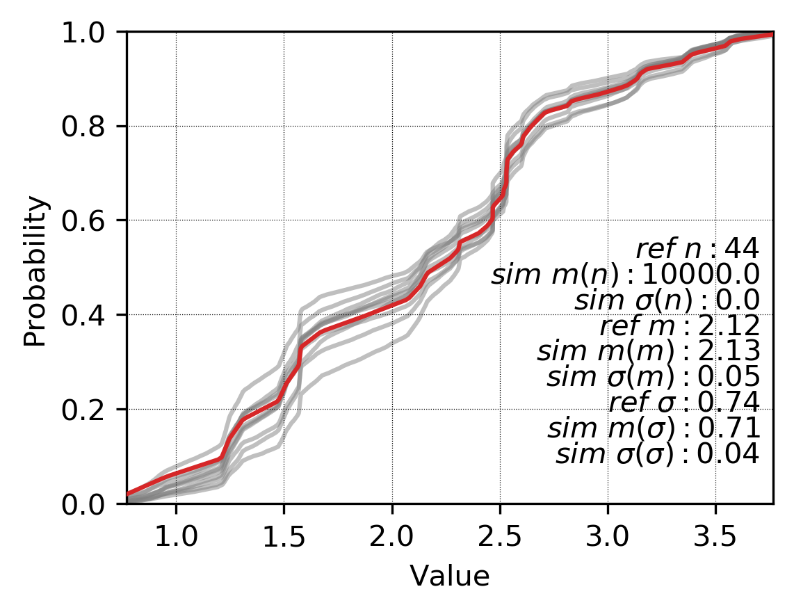
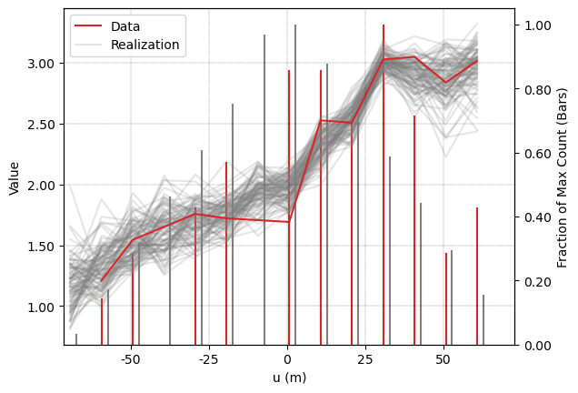
Histogram reproduction has a reasonable amount of variability between the realizations. Additional details on checking continuous simulated realizations are presented in the lesson Checking Continuous Variable Realizations - Mining. Although the trend is visually reproduced in section, this is verified by checking swath plots of all realizations along 045 degrees.

Practical Considerations

A primary consideration of trend modeling is the correct balance of variability between the trend model and the residuals. Many parameter choices such as the number of data and window size are subjective and ultimately control the variability of the trend. An over-fit trend will result in small stochastic residuals and too little uncertainty in the final model. It may be computationally expensive to test multiple trend models. An over-fit trend can lead to artificial destructuring of the variogram. The experimental variogram of the residuals should show some spatial structure and not be pure nugget.

Choosing to model a trend or not is an important consideration. Accounting for large-scale trends in the modeling workflow can significantly improve histogram and variogram reproduction when the spatial continuity of the underlying variable is long relative to the domain size. If the geologic nature of the trend is not well understood either conceptually or due to sparse data, modeling with a trend may not be appropriate. Sparse exploration data sets present real risks of trend over-fitting and residuals with too little variability.

Trend extrapolation should be handled with care. Different algorithms behave differently beyond the limits of the data. One approach could be to assume a constant trend value beyond a certain distance threshold (Pyrcz & Deutsch, 2014). Synthetic data may need to be added to control extrapolation, though some extrapolation is unavoidable as the margins of the domain are rarely sampled.

The example presented in this lesson is univariate. In the multivariate context, each variable is normal score transformed independently, and a trend of the normal scores is modeled for each variable. The workflow then includes a projection pursuit multivariate transform (PPMT) step after the SCT. Each variable has multiple forward transforms and multiple back transforms. The additional PPMT step ensures the variables are both uncorrelated with their respective trends and multivariate Gaussian.

Summary

Virtually all earth science data exhibit trend-like features. The goal of modeling with a trend is to satisfy the implicit assumption of stationarity in geostatistical simulation algorithms. Some subjective choices must be made during trend modeling. The practitioner must balance the variability explained by the trend with the variability of the residuals. The trend must be neither over- nor under-fit. The modern approach to modeling with a trend enforces independence between the random variable and the locally varying mean. The GMM based SCT removes the potential for binning artifacts during transformation. There is no chance of simulating negative values with the modern approach as the normal score variables are transformed directly.

A Note on Updates

On October 10, 2024, this Lesson was updated to reflect current best practice in trend modeling and add a reproducible notebook demonstrating the technique. This includes the use of swath plot verification of trend models and the assessment of detrended variograms and the nature of the destructing. These updates were made by Sebastian Sanchez, Ben Harding, and Ryan Barnett, all of Resource Modeling Solutions Ltd.. Upcoming publications by Thiago Alduini Mizuno and Clayton Deutsch of the University of Alberta in Stochastic Environmental Research and Risk Assessment supplement this Lesson.

References