Cite this lesson as: Gomes, C. G., & Boisvert, J. & Deutsch, C.V. (2022). Gaussian Mixture Models. In J. L. Deutsch (Ed.), Geostatistics Lessons. Retrieved from http://www.geostatisticslessons.com/lessons/gmm
Gaussian Mixture Models
Caio Cardoso Gomes
University of Alberta
Jeff Boisvert
University of Alberta
Clayton V. Deutsch
University of Alberta
August 15, 2022
Learning Objectives
- Review the theory and implementation of Gaussian Mixture Models (GMM)
- Understand the application of GMMs in Geostatistics
- Demonstrate application of the GMM with practical examples
Introduction
Mixture models are common for statistical modeling of a wide variety of phenomena. The premise is that a continuous distribution could be approximated by a finite mixture of Gaussian or normal densities (McLachlan & Peel, 2000). These Gaussian mixture models (GMMs) are considered to be semi-parametric distribution models since they are neither defined by a single parametric form nor based entirely on the data. They are usually fit with the Expectation-Maximization (EM) algorithm (Dempster, Laird, & Rubin, 1977) that is computationally efficient. The number of components used in the GMM can vary while having a simple form to the probability density function (McLachlan & Peel, 2000).
GMMs can reproduce complex univariate or multivariate distributions of geoscience datasets (Hadavand & Deutsch, 2020) and are applied for different purposes including (1) fitting probability density functions to permit the extraction of conditional distributions, (2) imputation of missing data to facilitate the use of techniques that require a full valued data table (Silva & Deutsch, 2018), and (3) clustering data into groups that are internally consistent and externally different.
The fundamentals required to understand GMMs are reviewed. Then, the application of GMMs to geostatistical modeling problems are explored, followed by small practical examples.
Gaussian Mixture Model (GMM)
A GMM is a probability density function (PDF) represented as a weighted linear combination of Gaussian component densities. A GMM is represented as (Reynolds, 2009): \[p(\mathbf{x}\vert \Psi) = \sum \limits _{i=1}^{M}\;{{w_i}\;g(\mathbf{x}\vert {\boldsymbol{\mu}}_{i},\, {\mathbf{\Sigma}}_{i})}\] where \(\mathbf{x}\) is a \(D\)-dimension continuous-valued data vector, \(w_i,i=1,...,M\), are the mixture weights, \(g(\mathbf{x}\vert { \boldsymbol{\mu}}_{i},\, {\mathbf{\Sigma}}_{i}),i=1,...,M\) are the Gaussian components, denoted by their mean \(\boldsymbol {\mu}_{i}\) and covariance matrix \({\mathbf{\Sigma}}\). \({\Psi}\) expresses the collection of all component parameters \({{\Psi} =( {w_i},\,{\boldsymbol{\mu}}_{i},\,\mathbf{\Sigma}_{i})}\), containing the weights, means, and covariance matrix for all Gaussian components.
An interactive illustration of univariate GMM.
The interactive figure shows an example of fitting a GMM to a univariate distribution. The user decides an appropriate number of Gaussian components (from one to eight in this example). The number of components is a key choice and is discussed below.
Implementation Details
Implementation of GMMs requires (1) deciding the number of Gaussian components for fitting, and (2) applying a fitting algorithm (conventionally the EM algorithm) with the desired covariance matrix type. The data considered in fitting the GMM may have declustering weights assigned to them to account for preferential sampling. Setting the marginal distribution independently of the data distribution is another alternative in the presence of non-representative data.
Expectation-Maximization (EM) Algorithm
The EM algorithm is widely used for iterative computation of maximum likelihood estimates (MLE) of distributions (Ng, Krishnan, & McLachlan, 2012). The EM algorithm is used to determine the parameters \({\Psi}\) (weights, means, and covariances) of the mixture model given some observed \({D}\)-dimensional \(\mathbf{x}\) data. This is achieved by maximizing likelihood, which determines the optimal parameters of the Gaussian components. The likelihood \(L({\Psi})\) is the joint probability of the observed data in terms of the statistical model parameters, as follows: \[{L({\Psi})={\prod_{i=1}^{n}}f(\mathbf{x_i};\Psi})\] The likelihood density function \(L({\Psi})= f(\mathbf{x};{\Psi})\) of the vector containing the unknown parameters \({\Psi}\) (\({\Psi^*}\)) is computed as (McLachlan & Peel, 2000): \(\partial\;{L}({\Psi})/{\partial\;({\Psi})}=0\) or in its more convenient logarithmic form: \(\partial\;{log L}\;({\Psi})/{\partial\;({\Psi})}=0\). The iterative EM algorithm used to calculate \({\Psi^*}\) consists of the following four steps (Saxena et al., 2017):
| Step | Action |
|---|---|
| 1. | Initialize the parameters \({\Psi}^{old}\): Usually \(k\)-means optimized centers are used as optimized |
| starting locations for running the first EM iteration. | |
| 2. | E-Step: Evaluate the conditional expectation for each Gaussian component given the current |
| parameters at every data sample. | |
| 3. | M-Step: Update the parameters \({\Psi}^{new}\) for maximization of likelihood to matching the |
| observed \(\mathbf{x}\) values. | |
| 4. | Check for convergence by comparing likelihood improvement of the initial parameters to the |
| updated parameters from M-step, additional details can be found in (Silva & Deutsch, 2015). |
Steps 2 through 4 are repeated until the likelihood stabilizes, indicating convergence to a local optimum (Silva & Deutsch, 2015). The tolerance for convergence is usually considered to be a maximum number of iterations (100 is standard) or can be based on the magnitude of the change between iterations (\(1x10^{-3}\) is standard).
Local Minima
In the context of GMM fitting, the EM algorithm is sensitive to the initialization of the Gaussian parameters \({\Psi}\) (Ng et al., 2012). A good practice that tends to avoid poor convergence is to use the optimized \(k\)-means centroids as the \(\boldsymbol{\mu}\) means for starting the first E-step (Ng et al., 2012). Another common strategy is to consider several runs of the EM algorithm, where the initial parameters \({\Psi}\) are randomly re-selected for each run; the optimum result of all random restarts is selected as the final set of parameters.
Covariance Matrix Type
The covariance matrix \({\mathbf{\Sigma}}_{i}\) models the statistical relationships between components, that is, their spread, correlation and orientation. A covariance matrix needs to be positive definite and can be built in different forms: full, this is the most flexible type as each Gaussian component has its own matrix (refer to (McLachlan & Peel, 2000)); diagonal, there are unique variances (diagonal terms) for each Gaussian component, but the correlation structure is preserved; tied, parameters are shared between Gaussian components (Pedregosa et al., 2011). Although the choice of covariance type might depend on the amount of data available and the intended use of the GMM, using the full covariance type is recommended for the majority of applications since it provides the greatest flexibility.
Optimal Number of Components
There is a trade off between over- and under-fitting. A small number of components are preferred to avoid over-fitting. Several methods are available to help determine an appropriate number of components including the likelihood ratio test (LRT) and the Bayesian information criterion (BIC) McLachlan & Rathnayake (2014). These metrics help assess sensitivity to the number of Gaussian components for fitting a distribution; however, the final decision of the number of Gaussian components rests with the practitioner.
Likelihood Ratio Test (LRT)
There is a threshold where increasing the number of Gaussian components in a finite mixture does not significantly improve the likelihood estimate. Multiple GMMs are fit with an increasing number of components. The improvement in the fits are compared and the difference or ratio between them serves as a useful metric. The test for this hypothesis is the LRT (McLachlan & Rathnayake, 2014), defined as \[{{\lambda}= {L}({\Psi}_{g0})/L({\Psi}_{g1})}\] for some \({g}_{1}>{g}_{0}\) (usually \(g1=g0+1\)), where \(g\) is the number of components and \({\lambda}\) is the likelihood ratio. For appropriately low values of \(\lambda\), \(g_0\) is disregarded as the optimal number of components in favor of \(g_1\). An hypothesis test could be relative to \(-2log{\lambda}\), to serve as evidence against \({g_0}\) (McLachlan & Rathnayake, 2014): \[-2log{\lambda}=2(logL({\Psi}_{g1})-logL({\Psi}_{g0}))\] It is usually more convenient to work with log-likelihood as the logarithmic form enhances the small differences generally seen in original likelihood values.
Bayesian Information Criterion (BIC)
A term is introduced to penalize a greater number of Gaussian components to avoid overfitting. The minimum score reflects the optimal number of components. Using more components results in a higher penalty: \[BIC= -2logL({\Psi})+ g logn\] where \(g\) is the number of Gaussian components in the model and \(n\) is the number of data points (McLachlan & Peel, 2000). The size of the dataset is also included in the penalty term although it is constant for any particular set of data.
Example Comparing BIC and LRT
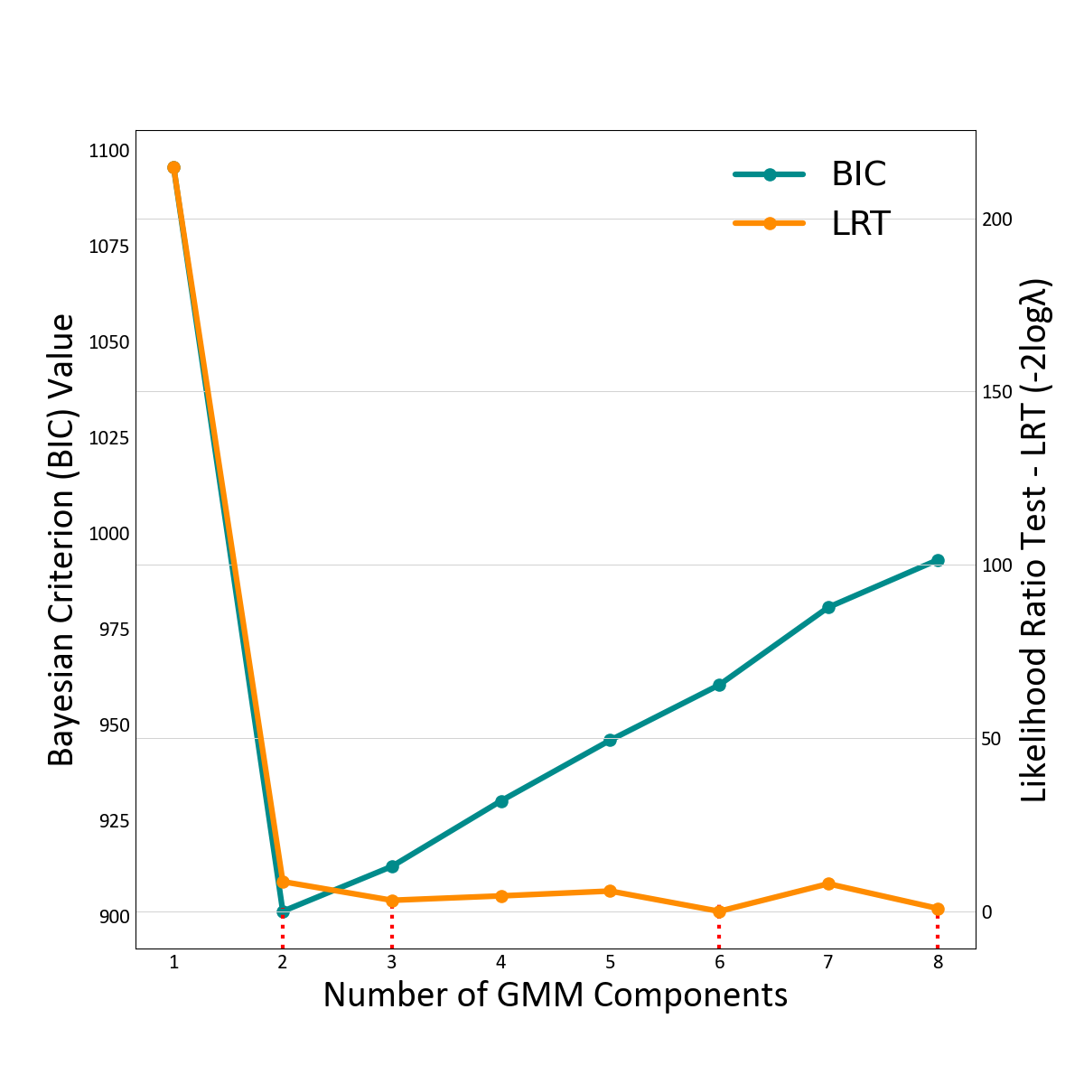
An example follows which demonstrates the use of LRT and BIC. The two metrics are compared in the context of defining the optimal number of components for the univariate fit example.

BIC values for this dataset reach their minimum when the number of components is equal to two, increasingly at a constant rate afterwards due to the penalty term, which is greater than the small likelihood improvement. The LRT reaches a local minimum with three components then decreases slightly. However, the absolute minimum LRT occurs when eight components are used, although at six components there is also a very low local minimum. Visual inspection of the fit in 2-D or 3-D may help determine the final number. A low number would often be preferred.
Applications in Geostatistics
Fitting Probability Distribution Functions (PDFs)
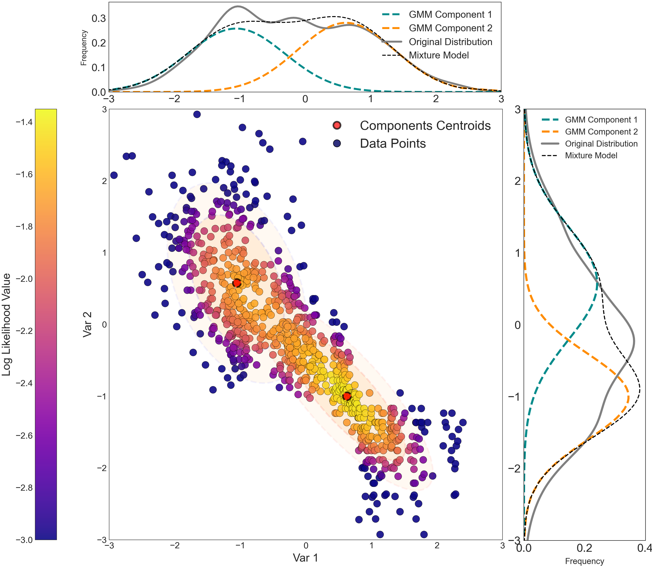
GMMs are useful for modeling complex, high dimensional data common in geoscience datasets (Sarkar, Melnykov, & Zheng, 2020). Generating smooth semiparametric models that fit the available data is an essential function of GMMs. The GMM modeled PDF can replace the original distribution for use in several geostatistical workflows. Consider the following bivariate distribution fit by a GMM with two components. Each component is parameterized by its mean, weights, and covariances, which combined produce the final mixture model. A GMM will show evidence of elliptical shapes (visible on the plot) that correspond to the constituent Gaussian components.

The Trend Modeling and Modeling with a Trend lesson offers one great example of GMMs primary application routes to modelling probability distributions. As explained by Harding & Deutsch (2021), GMM allow the bivariate relationship to be reproduced besides eliminating chances of binning artifacts in the Trend modelling work-flow.
Multiple Imputation
Multiple Imputation (MI) (Barnett & Deutsch, 2015; Enders, 2010; Little & Rubin, 2002) addresses an important and common geomodeling problem. Data sets are often missing measurements of some variables at some sample locations. Many geostatistical modeling workflows do not allow missing variables. MI is used to ‘fill in’ the values of variables missing at sample locations while honoring multivariate and spatial data distributions (Deutsch, Palmer, Deutsch, Szymanski, & Etsell, 2016).
Applications where this is important include principal component analysis (PCA), stepwise conditional transforms (SCT), minimum-maximum auto correlation factors (MAF) and projection-pursuit multiple transformation (PPMT) (Silva & Deutsch, 2018).
GMMs have been integrated in MI by Silva & Deutsch (2018) to build the conditional distributions from which to draw the imputed samples. This improves the accuracy of the imputed values and reduces the computational expense of alternatives such as kernel density estimation (Barnett & Deutsch, 2015; Silva & Deutsch, 2018).
Clustering
Clustering is a class of unsupervised machine learning techniques for grouping objects based on their similarities. Common techniques include hierarchical, partitioning, model-based and probability density-based methods (Saxena et al., 2017). GMMs can be used as a probabilistic density-based method for clustering. The Gaussian components are fit to the available data and discrete classes (clusters) are assigned based on the maximum likelihood of points belonging to each component (Martin, 2019; Sarkar et al., 2020; Saxena et al., 2017; Zhang, 2021).
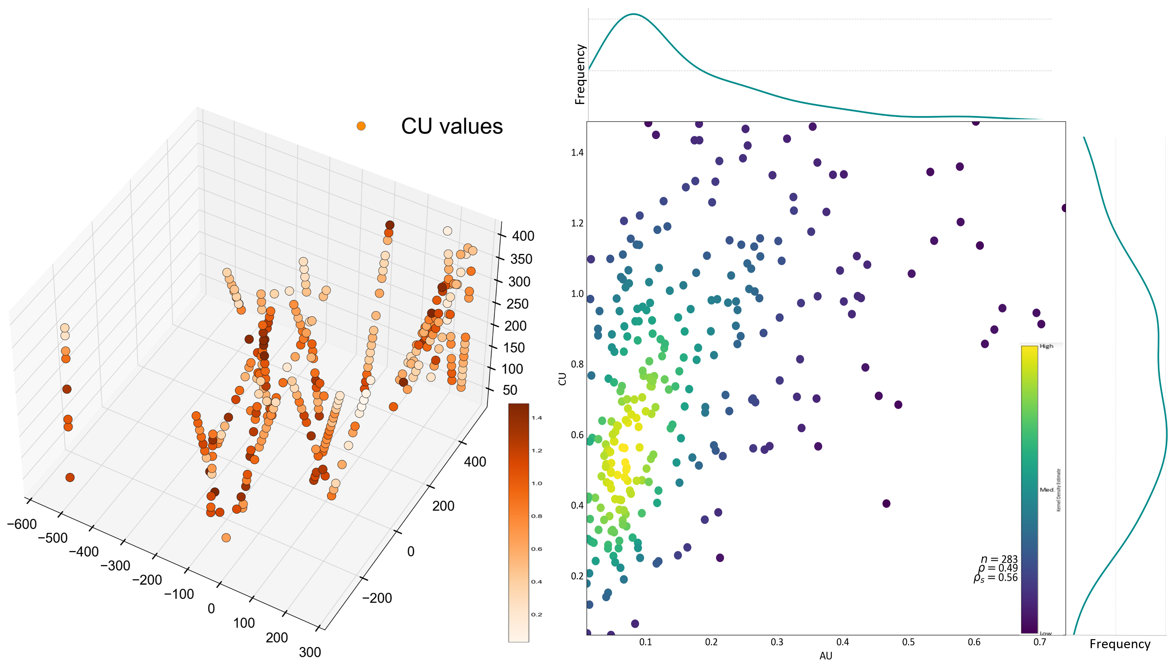
A porphyry gold-copper deposit is used to demonstrate the use of GMMs for clustering geological data sets. The 3-D map and the bivariate relationships are shown below. The optimal number of clusters for this dataset is also tested using the BIC and LRT metrics, which can be seen in the following interactive figure. It displays the location of the varying assigned clusters as the number of components change. GMM clustering considers the anisotropy in the data through the covariances; simple Euclidean clustering would always give isotropic ‘blob-like’ clusters. The GMM’s clusters strong anisotropies are visible in interactive figure below, especially for a higher number of components, say between 6 and 8.

An interactive illustration of GMM clustering.
The LRT and BIC methods yield multiple possibilities for the optimal number of components. BIC is minimized using three Gaussian kernels, while LRT is minimized with eight components; however, five also shows a significant local minimum.
Discussion
Gaussian Mixture Models (GMMs) play a role in fitting a distribution of n-dimensional data. There are some limitations. As explored by Zhang (2021), GMM clustering is sensitive to data transformation, spikes (recurrent values), below detection limit (BDL) samples, and outliers. A GMM may include overlapping components that provide a reasonable fit to the distribution, but may not be appropriate for clustering. GMMs are a widely used Machine Learning method, are easy to employ, and are accessible in many different software packages.