Learning Objectives

• Understand why multivariate Gaussian transforms are used for geostatistical modeling.
• Review essential steps of the projection pursuit multivariate transform (PPMT).
• Interpret PPMT results with data of varying dimensions to consolidate understanding of the technique.

Introduction

Linear decorrelation transforms, such as principal component analysis (PCA) and min/max autocorrelation factors (MAF) are popular geostatistical tools for modeling multiple geological variables. Readers unfamiliar with these methods are encouraged to review the associated lessons as they provide the foundation for methods in this lesson. Linear decorrelation transforms are commonly applied within geostatistical simulation workflows that follow five primary steps:

1. Standardization or a normal score transform is used to center the variables and improve interpretability
2. A linear transform is used to decorrelate the variables
3. A normal score transform is applied to the decorrelated variables, making them univariate Gaussian
4. Realizations of the transformed variables are simulated independently, assuming they follow the uncorrelated multivariate Gaussian (multiGaussian) distribution
5. The normal score, linear and standardization back-transforms restore the original correlation and units to the realizations

There are potential issues with this workflow. First, the normal score transform may re-introduce correlation to the decorrelated variables. Second, and more significantly, dependence may exist in the decorrelated variables. A correlation coefficient parameterizes a multiGaussian distribution such as the schematic illustration below, but does not parameterize data with complexities such as non-linearity, heteroscedasticity and constraints.

Any dependence that is not parameterized by the correlation coefficient will not be removed by linear decorrelation transforms. If remnant dependence is significant when applying Step 3 above, the back-transformed realizations are unlikely to reproduce the original multivariate dependencies, as well as univariate properties such as the histogram. This motivates multiGaussian transforms, which facilitate the following workflow:

1. A multiGaussian transform makes the variables uncorrelated and multiGaussian
2. Realizations of the transformed variables are simulated under the assumption of independence
3. The multiGaussian back-transform restores the original multivariate dependencies and units to the realizations

The key to this workflow is that an uncorrelated and multiGaussian distribution is independent by definition so that the assumption in Step 2 is valid. Unlike linear decorrelation, the multiGaussian transform removes multivariate complexities before reintroducing them to simulated realizations. This workflow was introduced by (Leuangthong & Deutsch, 2003), where the stepwise conditional transform (Rosenblatt, 1952) was used.

Although suitable in some cases, the binning nature of stepwise often creates challenges for greater than 2 to 4 variables. This served as primary motivation for the projection pursuit multivariate transform (Barnett, Manchuk, & Deutsch, 2014), which applies a modified form of the transform that is internal to projection pursuit density estimation (Friedman, 1987; Hwang, Lay, & Lippman, 1994). Relative to stepwise, the PPMT may be applied to additional variables and requires fewer implementation parameters. This lesson begins by outlining the major steps of the PPMT. After demonstrating the transform, practical considerations relating to its use within a multiGaussian simulation workflow are discussed.

Transform Steps

The PPMT is composed of two major steps, pre-processing and projection pursuit. Pre-processing is used to make the data marginally Gaussian and remove linear dependence, before projection pursuit makes the data multiGaussian through removing complex dependence. Readers are referred to (Barnett et al., 2014) and (Barnett, Manchuk, & Deutsch, 2016) for additional information.

Pre-processing

Consider \(k\) geological variables \(Z_1,...,Z_k\) that are sampled at \(n\) locations to provide the data matrix \(\mathbf{Z}: z_{\alpha,i}, \alpha=1,...,n, i=1,...,k\). The first pre-processing step applies the normal score transform (Bliss, 1934; Verly, 1983). Although it is used extensively in geostatistics, the normal score transform is formally defined and schematically illustrated below since it is also used within projection pursuit: \[\mathbf{Y}: y_{\alpha,i} = G^{ - 1} \left( F_i (z_{\alpha,i} ) \right), \text{ for } \alpha = 1,...,n, i = 1,...,k\]

where probabilities \(p\) are matched between the cumulative distribution function (CDF) of each variable \(F_i\) and the standard Gaussian distribution \(G\). The resulting \(\mathbf{Y}\) data is univariate standard Gaussian (or standard normal), which beyond being a targeted final data property, also improves robustness of the covariance matrix that is calculated in the next step. The standard Gaussian distribution has a mean of zero and variance of one, which simplifies calculations that follow.

The second pre-processing step is data sphereing, which transforms the data to be uncorrelated with unit variance. Begin by calculating the covariance matrix: \[\boldsymbol{\Sigma}: C_{i,j}=\frac{1}{n} \sum_{\alpha=1}^n y_{\alpha,i}^2, \text{ for } i,j=1,...,k \]

Spectral decomposition of \(\boldsymbol{\Sigma}\) is then performed yielding the orthogonal eigenvector matrix \(\mathbf{V}:v_{i,j},i,j=1,...,k\) and the diagonal eigenvalue matrix \(\mathbf{D}:d_{i,i},i=1,...,k\): \[\boldsymbol{\Sigma} = \mathbf{V}\mathbf{D}\mathbf{V}^T\]

The sphereing transform (specifically, spectral decomposition sphereing) is given as: \[\mathbf{X}= \mathbf{YVD}^{-1/2}\mathbf{V}^T\]

The rotated data has an identity covariance matrix, meaning that \(X_1,...,X_k\) have a variance of one and are uncorrelated. The \(\mathbf{V}^T\) term rotates the variables back to their original basis, which minimizes the mixing of \(Y_1,...,Y_k\) amongst \(X_1,...,X_k\), through maximizing the loading of the \(Y_i\) variable onto its corresponding \(X_i\) variable. Similarly, subsequent projection pursuit transforms the variables to be multiGaussian in a manner that minimizes their mixing. This ‘gentle’ transformation of the data means that unique characteristics of the original variables (e.g., their respective variograms) are relatively well-preserved in the uncorrelated multiGaussian data, making their reproduction more likely following independent geostatistical simulation and back-transformation.

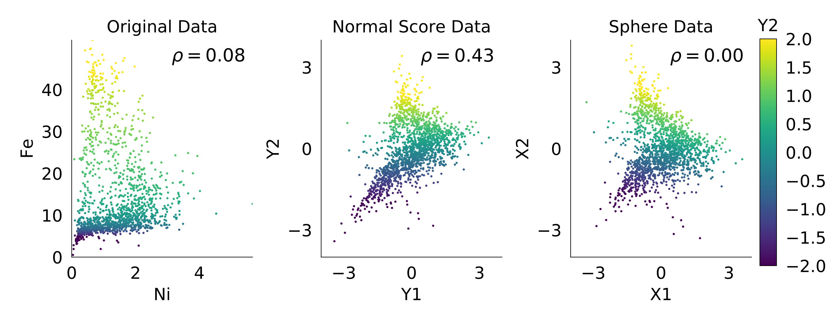
The PPMT is demonstrated with nickel laterite data, where only two variables are used initially for visual clarity. The scatter plots below display the pre-processing steps, where nickel (Ni) and iron (Fe) are normal score and sphere transformed. The influence of outlier values on the correlation coefficient (\(\rho\)) is evident when comparing the original and normal score data. Sphereing is shown to remove correlation, but not the complex dependencies that exist between Ni and Fe. These complexities are addressed with projection pursuit.

Projection Pursuit

Consider a \(k\)x\(1\) unit length vector \(\boldsymbol{\theta}\) and the associated projection of the data upon it, \(\mathbf{p} = \mathbf{X}\boldsymbol{\theta}\). Any \(\boldsymbol{\theta}\) should yield a \(\mathbf{p}\) that is univariate Gaussian if \(\mathbf{X}\) is multiGaussian. With this in mind, define a test statistic (termed projection index) \(I(\boldsymbol{\theta})\), which measures univariate non-Gaussianity. For any \(\boldsymbol{\theta}\) where the associated \(\mathbf{p}\) is perfectly Gaussian, \(I(\boldsymbol{\theta})\) is zero. Projection pursuit uses an optimized search to find the \(\boldsymbol{\theta}\) that maximizes \(I(\boldsymbol{\theta})\), meaning that it finds the vector with the most non-Gaussian projection of \(\mathbf{X}\). Readers are referred to (Friedman, 1987) for additional details on the projection index and optimized search.

After determining the optimum \(\boldsymbol{\theta}\), \(\mathbf{X}\) is transformed to \(\mathbf{\tilde X}\), where the projection \(\mathbf{\tilde p} = \mathbf{\tilde X}\boldsymbol{\theta}\) is standard Gaussian. This is accomplished using several steps. Begin by calculating the orthogonal matrix:

\[\mathbf{U} = [\boldsymbol{\theta} ,\boldsymbol{\phi} _1,\boldsymbol{\phi} _2 ,...,\boldsymbol{\phi} _{k - 1} ]\]

where each \(k\)x\(1\) unit vector \(\boldsymbol{\phi} _i\) are calculated using the Gram-Schmidt algorithm (Reed & Simon, 1972). The multiplication of \(\mathbf{X}\) and \(\mathbf{U}\), results in a transformation where the first column is the projection \(\mathbf{p}=\mathbf{X}\boldsymbol{\theta}\):

\[\mathbf{XU} = [\mathbf{p},\mathbf{X}\boldsymbol{\phi} _1,\mathbf{X}\boldsymbol{\phi} _2,...,\mathbf{X}\boldsymbol{\phi} _{k - 1}]\]

Next, let \(\Theta\) be a transformation that yields a standard Gaussian projection \(\mathbf{\tilde p}\), while leaving the remaining orthogonal directions intact:

\[\Theta (\mathbf{XU}) = [\mathbf{\tilde p},\mathbf{X}\boldsymbol{\phi} _1,\mathbf{X}\boldsymbol{\phi} _2,...,\mathbf{X}\boldsymbol{\phi} _{k - 1}]\]

To be clear, \(\Theta\) is simply a normal score transform of the first column of \(\mathbf{XU}\). Multiplying this result by \(\mathbf{U}^T\) returns \(\Theta (\mathbf{XU})\) to the original basis:

\[\mathbf{\tilde X} = \Theta (\mathbf{XU}) \mathbf{U}^T\]

The transformed multivariate data \(\mathbf{\tilde X}\) will now yield a Gaussian projection along \(\boldsymbol{\theta}\) and therefore have a projection index of \(I(\boldsymbol{\theta})=0\). The optimized search for the maximum projection index may be repeated on \(\mathbf{\tilde X}\) to find other complex directions.

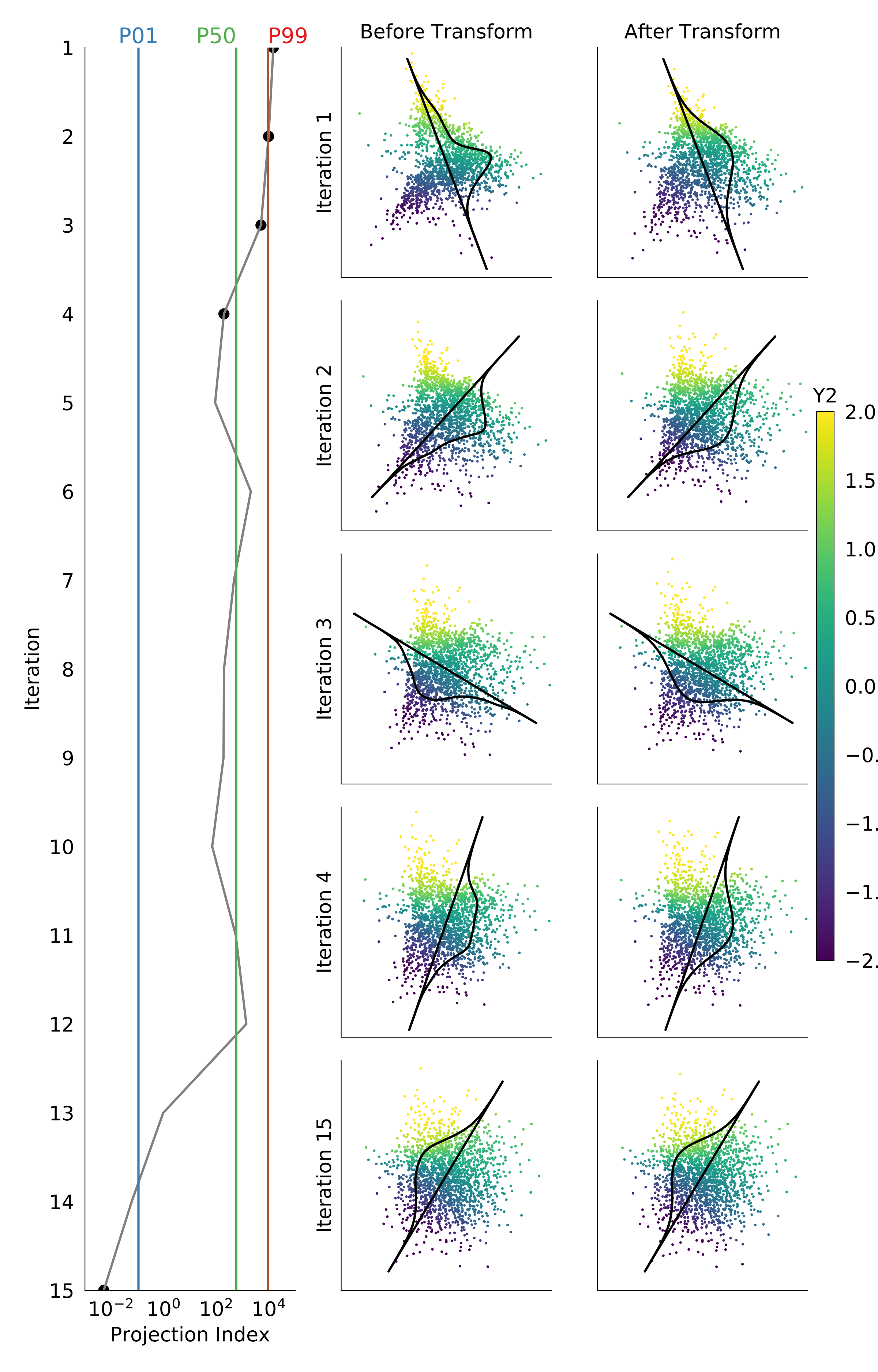
Scatter plots in the multi-panel figure below display select projection pursuit iterations, beginning from the sphered data that was displayed above. Readers using a web-browser may view each iteration with the interactive figure that follows. The orientation of the displayed probability density function (PDF) corresponds with the optimum \(\boldsymbol{\theta}\), where the PDF is shown to be non-normal and normal before and after transformation. The \(Y_2\) coloring (normal score Fe values) is used to understand the relative movement of data in each transform, displaying that the data is made multiGaussian with minimal mixing. The left panel displays progression of the projection index \(I(\boldsymbol{\theta})\) on a logarithmic axis, showing that non-Gaussianity of the projection greatly decreases following 15 iterations. The iterations show an increase in the projection index, which correspond primarily with a local optimum being found on the previous iteration. The highlighted percentiles correspond with stopping criteria that are described in the next section.

Scatter and projection of the data. Use the slider at the bottom to view each iteration, before and after transformation.

Stopping Criteria

Choosing the target value to which the projection index \(I(\boldsymbol{\theta})\) must descend is not straightforward. Increasing \(k\) dimensions make the discovery and resolution of complexity in the data more difficult. A smaller number of \(n\) observations make the projections less reliable for detecting meaningful multivariate structure. These characteristics are also observed in random samples from a multiGaussian distribution, where reducing \(n\) and increasing \(k\) creates an increasingly non-Gaussian random sample.

Drawing on this parallel, the target \(I(\boldsymbol{\theta})\) for PPMT stopping could be determined by random samples from a multiGaussian distribution. A bootstrapping algorithm is implemented, where \(m\) distributions of matching \(k\) and \(n\) are randomly sampled from the Gaussian CDF. A projection index value \(I(\boldsymbol{\theta})\) is then calculated for all \(m\) distributions along \(k\) random orthogonal unit vectors. This process yields an \(m\)x\(k\) distribution of projection indices, which may be used for targeting a very Gaussian distribution (P01 percentile) or barely Gaussian distribution (P99). For example, targeting the P01 percentile would cause the PPMT to terminate after the 14th iteration according to the figure above. This means that the transformed data is more multiGaussian that 99% of the randomly generated multiGaussian distributions.

Nickel Laterite Example

The PPMT was demonstrated above with only \(k=2\) variables to aid in visual interpretation. It may be used effectively, however, for transforming data of larger \(k\) to be uncorrelated and multiGaussian. The Ni and Fe variables that a were previously presented, are drawn from a Ni laterite dataset that also includes SiO₂, MgO, Co and Al₂O₃. In particular, it is important that geostatistical models reproduce the complex relationship that exists between Ni, Fe, SiO₂, and MgO.

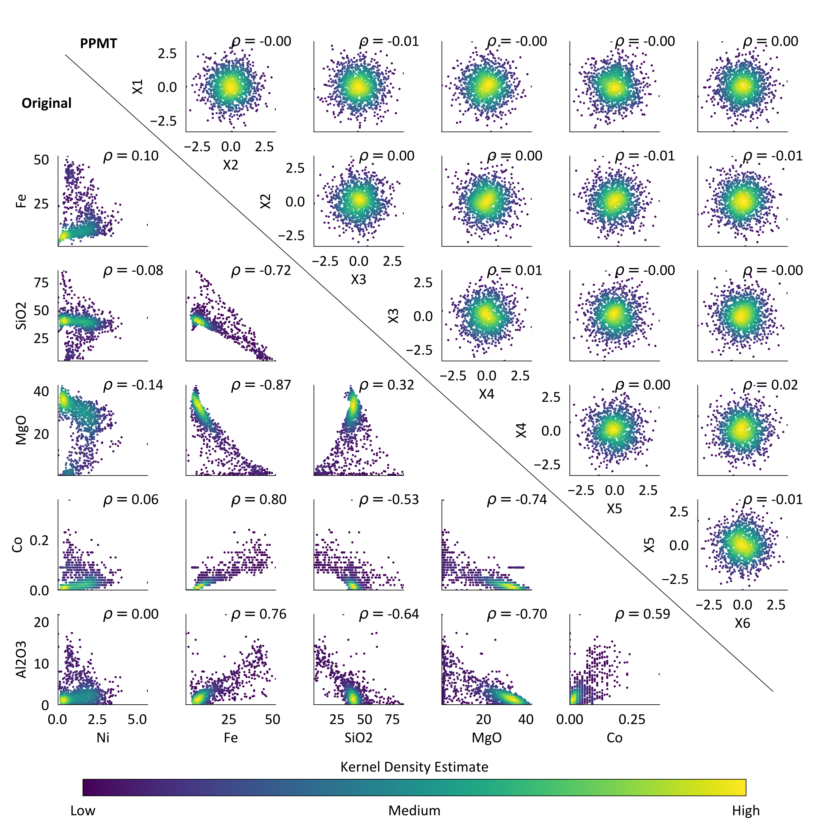
Scatter between these original variables is displayed in the lower triangle of the below plot, where they are colored by the associated Gaussian kernel density estimate to provide an indication of the multivariate point densities. Observe that the complex relations between these variables are not parameterized by the displayed correlation coefficients. Applying linear decorrelation transforms would remove their correlation, but would not make them independent.

The PPMT was applied with a projection index target of the P01 percentile, as well as a maximum of 150 iterations in case that target cannot be achieved. The algorithm terminated after 150 iterations, having only reached the P13 percentile. Kernel density coloring of the transformed scatter plots (upper triangle) approximates the multiGaussian density contours, while the majority of correlation coefficients are zero to the second decimal. Given that variables are more multiGaussian than 87% of randomly generated multiGaussian distributions, while being virtually uncorrelated, it is reasonable to simulate them under an assumption of independence.

Practical Considerations

There are several practical considerations for using the PPMT in simulation workflows, as discussed in (Barnett et al., 2016). Both the PPMT transformed data and independently simulated realizations are assumed to follow the standard multiGaussian distribution. Applying the PPMT back-transform should then provide realizations that match the original multivariate distribution. Unfortunately, simulated realizations may not be standard Gaussian. For example, a large variogram range relative to the model domain size leads to realizations with a variance less than one. The resulting mismatch of data and realization distributions in Gaussian units will lead to a mismatch of distributions in original units following back-transformation. Realizations will not reproduce the original multivariate distribution and may not reproduce its marginal distributions (e.g, histograms). Applying histogram corrections (Journel & Xu, 1994) in Gaussian and/or original space may be necessary in such cases.

The variogram model that is used for simulating each PPMT transformed \(\tilde X_i\) variable should be fit to the corresponding normal score transformed \(Y_i\) variable (output from the first pre-processing step). Although non-intuitive, this is often necessary since the removal of multivariate dependence between regionalized variables can lead to destructuring of their spatial continuity. Fitting variogram models to the normal score transformed variables has been found to provide the most effective reproduction of the original variograms following simulation and back-transformation. This approach is reasonable since each \(Y_i\) is heavily loaded on \(\tilde X_i\).

Although the PPMT may be applied to data of any reasonable \(n\) samples and \(k\) dimensions, its modeling workflow generally performs better with decreasing \(k\) and increasing \(n\). With a relatively large \(k\) (e.g., \(k>10\)) and relatively small \(n\) (e.g., \(n<1000\)), sampling of multivariate space becomes very sparse. A simulated node may then be located in an area of Gaussian space that is far from the nearest transformed data, increasing the likelihood that the interpolation that is implicit to the back-transform leads to problematic results (e.g., values beyond visual constraints in original space). Using the Gibbs sampler (Geman & Geman, 1984) to populate multivariate space with additional pseudo-data is recommended if such problems are observed. This pseudo-data is input to the PPMT for improving the noted issue, although it is not used for model conditioning.

Summary

MultiGaussian transforms are powerful tools for geostatistical modeling. Multivariate dependencies, including complex relations, are removed by these techniques, allowing for simulation under a valid assumption of independence. The back-transform then restores original units and complexity. Linear decorrelation transforms only remove linear dependence and are unlikely to reproduce complex multivariate features, although they remain appropriate in the absence of such features.

The PPMT transform was discussed in this lesson, which applies a modified version of the multiGaussian transformation that is internal to projection pursuit density estimation. Several important considerations were then listed for applying the PPMT within simulation workflows.

References