Learning Objectives

• Understand principal component analysis (PCA) within the context of multivariate geostatistical modeling.
• Review essential PCA theory relating to decorrelation and dimension reduction.
• Interpret PCA results with data of varying dimensions to consolidate understanding of the technique.

Introduction

Principal component analysis (PCA) (Hotelling, 1933; Pearson, 1901) is a dimension reduction and decorrelation technique that transforms a correlated multivariate distribution into orthogonal linear combinations of the original variables. PCA is a useful geostatistical modeling tool for two primary reasons:

1. Multivariate data, consisting of multiple correlated geological variables, are transformed by PCA to be uncorrelated. Independent geostatistical modeling of the decorrelated variables then proceeds, before the PCA back-transform restores the original correlation to the modeled variables.
2. PCA may be used for dimension reduction in the above framework. Independent geostatistical modeling proceeds on a subset of the decorrelated variables, before the PCA back-transform provides models of all original variables.

PCA could be used to gain a deeper understanding of underlying latent factors, but in geostatistics these two reasons prevail. It was first applied to geostatistical modeling in this manner by (Davis & Greenes, 1983), with more recent examples from (Barnett & Deutsch, 2012) and (Boisvert, Rossi, Ehrig, & Deutsch, 2013). This lesson begins with a description of the data processing and covariance calculations that are necessary prior to applying PCA. Essential PCA theory is then outlined and demonstrated with a small example, before demonstrating it with a larger geochemical dataset.

Data Pre-processing and Covariance Calculation

Consider \(k\) geological variables \(Z_1,\ldots,Z_k\) that will be simulated across a stationary domain \(A\). Conditioning data is given as the matrix \(\mathbf{Z}: z_{\alpha, i}, \alpha=1,\ldots,n, i=1,\ldots,k\), where \(n\) is the number of samples. The \(\mathbf{Z}\) data is assumed to be representative of the domain \(A\), so that parameters may be calculated experimentally. Variables must be transformed to have a mean of zero (termed centered) before applying PCA or any linear rotation. It is also recommended that the variables be transformed to have variance of one, as this improves the interpretability of subsequent PCA results. Standardization of the geological variables is therefore used as a pre-processor to PCA: \[ \mathbf{Y}: y_{\alpha,i} = \frac{(z_{\alpha,i}- \mu_i)}{ \sigma_i}, \text{ for } \alpha=1,\ldots,n,i=,1,\ldots,k\]

where \(\mu_i=1/n\sum_{\alpha=1}^n z_{\alpha,i}\) is the mean of \(Z_i\) and \(\sigma_i^2 = 1/n\sum_{\alpha=1}^n z_{\alpha,i}^2 - \mu_i^2\) is the variance of \(Z_i\). Each standardized \(Y_i\) variable has a mean of zero and a variance of one. PCA revolves around the covariance matrix \(\boldsymbol{\Sigma}\) of the \(\mathbf{Y}\) data, which is calculated as:
\[ \boldsymbol{\Sigma}: C_{i,j}=\frac{1}{n} \sum_{\alpha=1}^n y_{\alpha,i} \cdot y_{\alpha,j}, \text{ for } i,j=1,\ldots,k\]

The \(\boldsymbol{\Sigma}\) values parameterize the multivariate system of the \(\mathbf{Y}\) data in terms of linear variability and dependence. Diagonal entries \(C_{i,i}\) are the variance of each \(Y_i\). Off-diagonal entries \(C_{i,j}, i \ne j\) are the covariance between \(Y_i\) and \(Y_j\). These covariances are also correlations since each \(Y_i\) has a variance of one.

PCA results are subject to the accuracy of \(\boldsymbol{\Sigma}\). If the calculated sample \(\boldsymbol{\Sigma}\) is not representative of the true population covariances, then PCA will not make the population uncorrelated in reality. For example, the covariance calculation is very sensitive to outlier values. Careful exploratory analysis should be performed to detect and remove erroneous outliers from the data prior to the covariance calculation.

The familiar normal score transform may be considered in the place of standardization, as normal scores have a mean of zero, variance of one and no univariate outliers. This will likely improve robustness of the covariance calculation and linear rotation, although multivariate outliers may persist to have adverse consequences. The normal score transform is non-linear, which has implications for estimation. Back-transforming normal score estimates directly will introduce a bias, although transforming a series of quantiles, as in PostMG (Lyster & Deutsch, 2004), solves this issue.

PCA Transform

The first step of PCA performs spectral decomposition of \(\boldsymbol{\Sigma}\), yielding the eigenvector matrix \(\mathbf{V}:v_{i,j},i,j=1,\ldots,k\) and the diagonal eigenvalue matrix \(\mathbf{D}:d_{i,i},i=1,\ldots,k\): \[\boldsymbol{\Sigma} = \mathbf{VDV}^T\]

The PCA transform is then performed through the matrix multiplication of \(\mathbf{Y}\) and \(\mathbf{V}\): \[\mathbf{P}= \mathbf{YV}\]

This rotates the multivariate data so that the resultant principal components in \(\mathbf{P}\) are uncorrelated. Multiplying \(\mathbf{P}\) by the transpose of \(\mathbf{V}\) rotates the data back to \(\mathbf{Y}\), providing the back-transform that may be used for simulated realizations of the principal components: \[\mathbf{Y}= \mathbf{PV}^T\]

The eigenvector matrix may be thought of as a rotation matrix, providing a new basis where the correlated data are made orthogonal. The linear matrix multiplication of \(Y_1,\ldots,Y_k\) with the \(i^{th}\) column of \(\mathbf{V}\) provides the \(P_i\) principle component. Hence, each principal component is a linear combination of the original variables, explaining the nature of the linear rotation terminology.

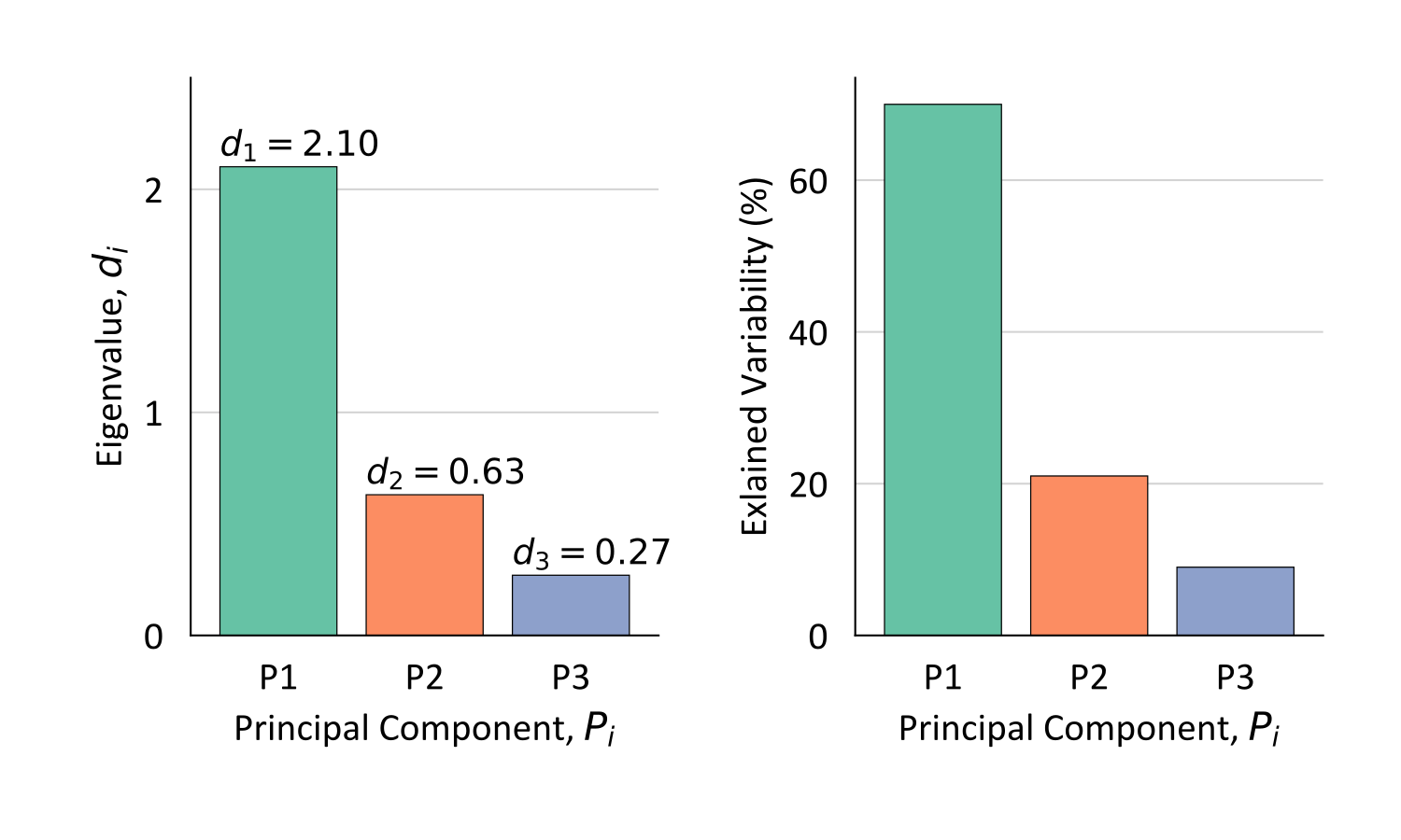
Each \(d_{i,i}\) entry corresponds with the variance of \(P_i\), while also measuring the variability that \(P_i\) explains about the \(Y_1,\ldots,Y_k\) multivariate system. More specifically, the percentage variability that \(P_i\) explains about the \(Y_1,\ldots,Y_k\) is calculated as \(d_{i,i}/\sum_{j=1}^kd_{j,j} \cdot 100\), or \(d_{i,i}/\textrm{tr}(\mathbf{D})\cdot 100\). The component \(P_1\) explains the most variability, \(P_2\) explains the second most, and so on.

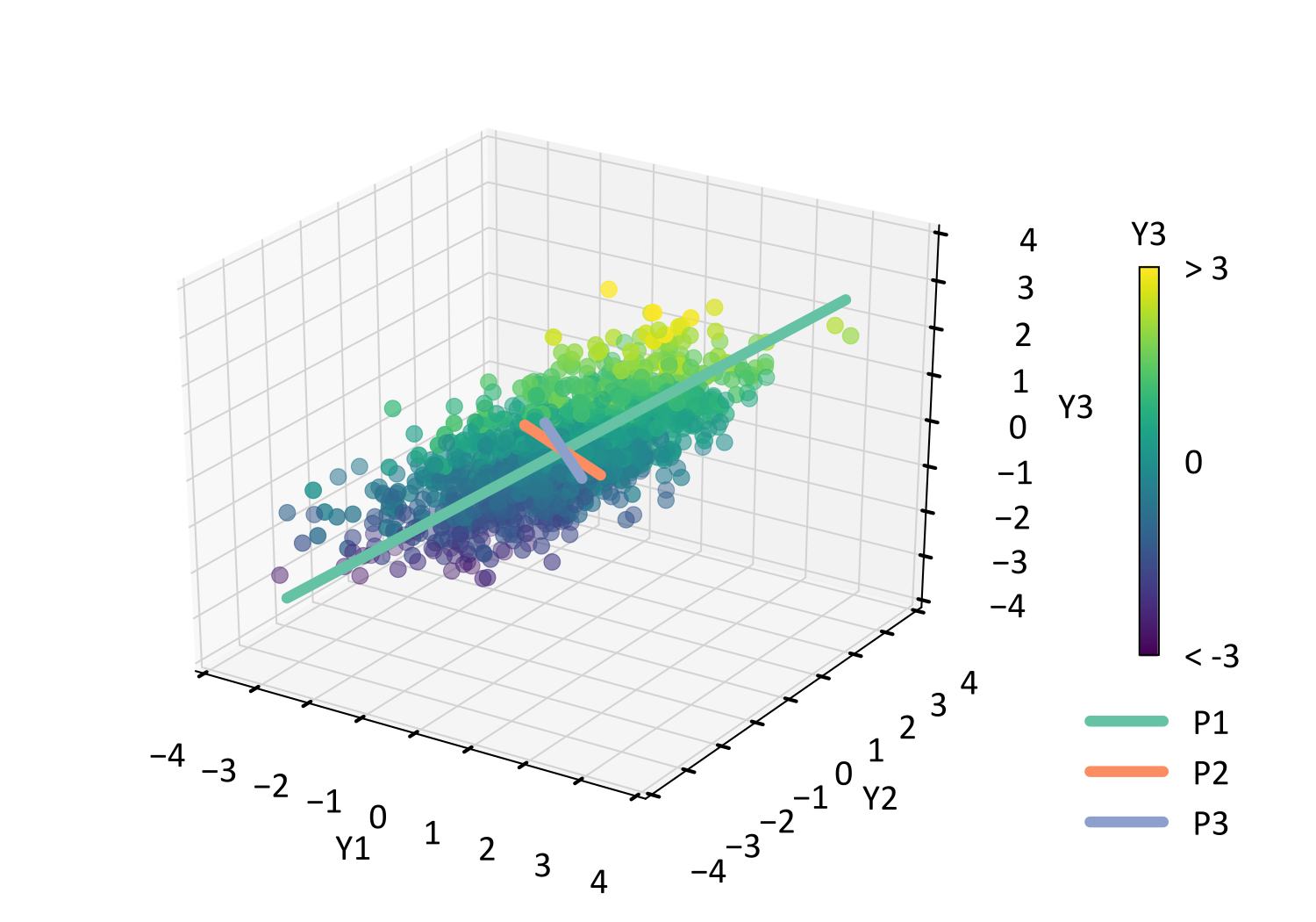
PCA is demonstrated using a small \(k=3\) example. The scatter plot of the \(Y_1,\ldots,Y_3\) data is overlain with the \(P_1,\ldots,P_3\) principal component vectors, which correspond with each column of \(\mathbf{V}\) and display the rotation basis (e.g., axes of principal components). The vector lengths are scaled according to the associated eigenvalues, which are also displayed in the bar chart below.

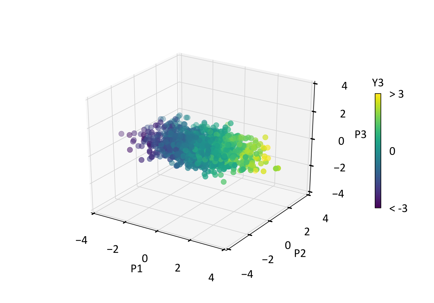
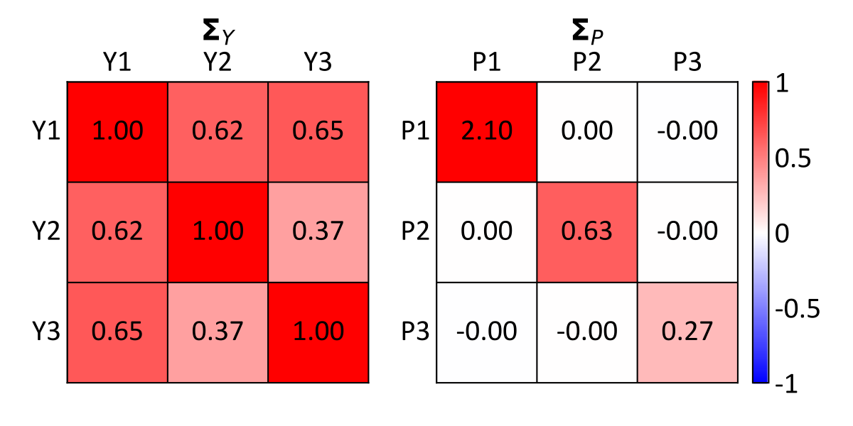
Following transformation, the below scatter plot displays \(\mathbf{P}\) data in the rotated basis, where the greatest variance exists visibly in the \(P_1\) dimension. Scatter plots in this lesson are colored according to their associated \(Y_3\) value, which indicates how each data point is rotated and shifted by the various transformations. The nature of this PCA rotation may be understood by comparing the \(\mathbf{Y}\) and \(\mathbf{P}\) scatter plots. The displayed covariance matrices confirm that: 1) the data are made uncorrelated according to the off-diagonal entries and 2) the principal components contain decreasing variance according to eigenvalues in the diagonal entries.

Dimension Reduction

Since eigenvalues measure the variability that each principal component contributes to the original multivariate system, practitioners may consider discarding insignificant components from subsequent geostatistical modeling. This is not utilized often in practice, but is available when an infeasibly large number of variables must be modeled. Consider that the \(l\) most important principal components are selected for simulation across \(N\) model nodes, where \(l < k\). Letting the resulting realization values be the \(Nxl\) matrix \(\mathbf{P}'\), the PCA back-transform is simply modified by multiplying \(\mathbf{P}'\) with the \(l\) rows of \(\mathbf{V}^T\). The multiplication of these \(N\) x \(l\) and \(lXk\) matrices yields the \(N\) x \(k\) matrix \(\mathbf{Y}\) of the standardized variable realizations.

The effectiveness of this dimension reduction scheme relates to the magnitude of variance that the removed principal components explain. If the associated eigenvalues are vanishingly small, then removal of those principal components should not have a significant impact on simulation results. The figure below demonstrates the PCA back-transform of \(l=1\) and \(l=2\) of the \(k=3\) components. Rather than a simulated realization, the transformed \(\mathbf{P}\) data is simply being back-transformed. The true standardized data values are compared with the back-transformed values, where perfect reproduction of the original values would be achieved if back-transforming all \(k=3\) components, leading to all scatter falling on a 45 degree line and correlation of \(\rho=1\). Scatter about the 45 degree line represents imperfect reproduction of the data, resulting from the loss of variability that would have been explained by the removed principal component(s). In this case, each principal component explains a significant amount of variability, so that the impact of their removal is substantial. Smaller eigenvalues can be expected as \(k\) grows larger, making the use of dimension reduction more effective.

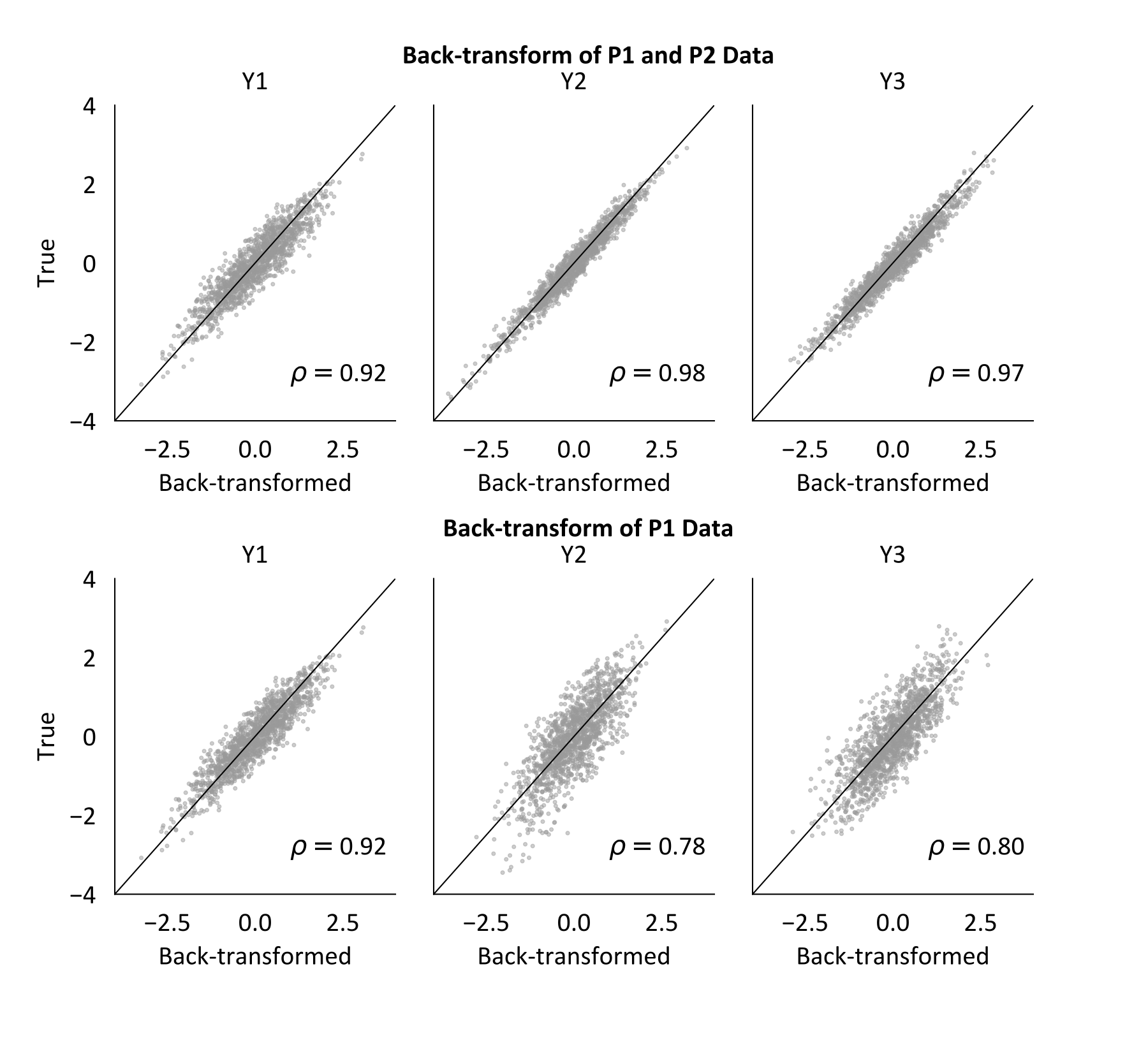
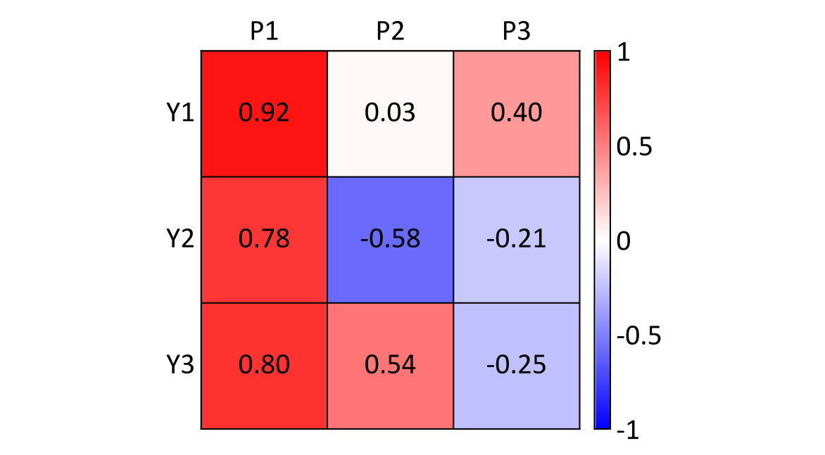
It is interesting to note that \(Y_1\) reproduction is virtually identical whether using \(l=1\) or \(l=2\) principal components, whereas the reproduction of \(Y_2\) and \(Y_3\) is significantly improved. This relates to the nature of the rotation and how the original variables are loaded onto the principal components. A loading \(\rho'(Y_i,P_j)\) describes how important the \(P_j\) principal component is for characterizing the \(Y_i\) variability. It is calculated as: \[\rho'(Y_i ,P_j ) = v_{i,j} \cdot d_{j,j} = \rho (Y_i ,P_j ) \cdot \sigma_i \]

This shows that a loading is the product of eigenvectors \(v_{i,j}\) and eigenvalues \(d_{i,i}\), though it may be more intuitively thought of as the correlation \(\rho\) between the original and transformed variables, scaled by the standard deviation of \(Y_i\). When working with standardized data, as we are here, a loading is simply the correlation between the \(Y_i\) original variable and the \(P_j\) principal component, \(\rho'(Y_i,P_j) = \rho(Y_i ,P_j )\). Inspecting the loadings of this transformation, observe that \(P_2\) is virtually uncorrelated with \(Y_1\). That is why the results above show that the inclusion and exclusion of \(P_2\) in the back-transform yields virtually identical results for \(Y_1\). All of the original variables are loaded most heavily on \(Y_1\), which is expected since it explains the majority of their variability.

Geochemical Example

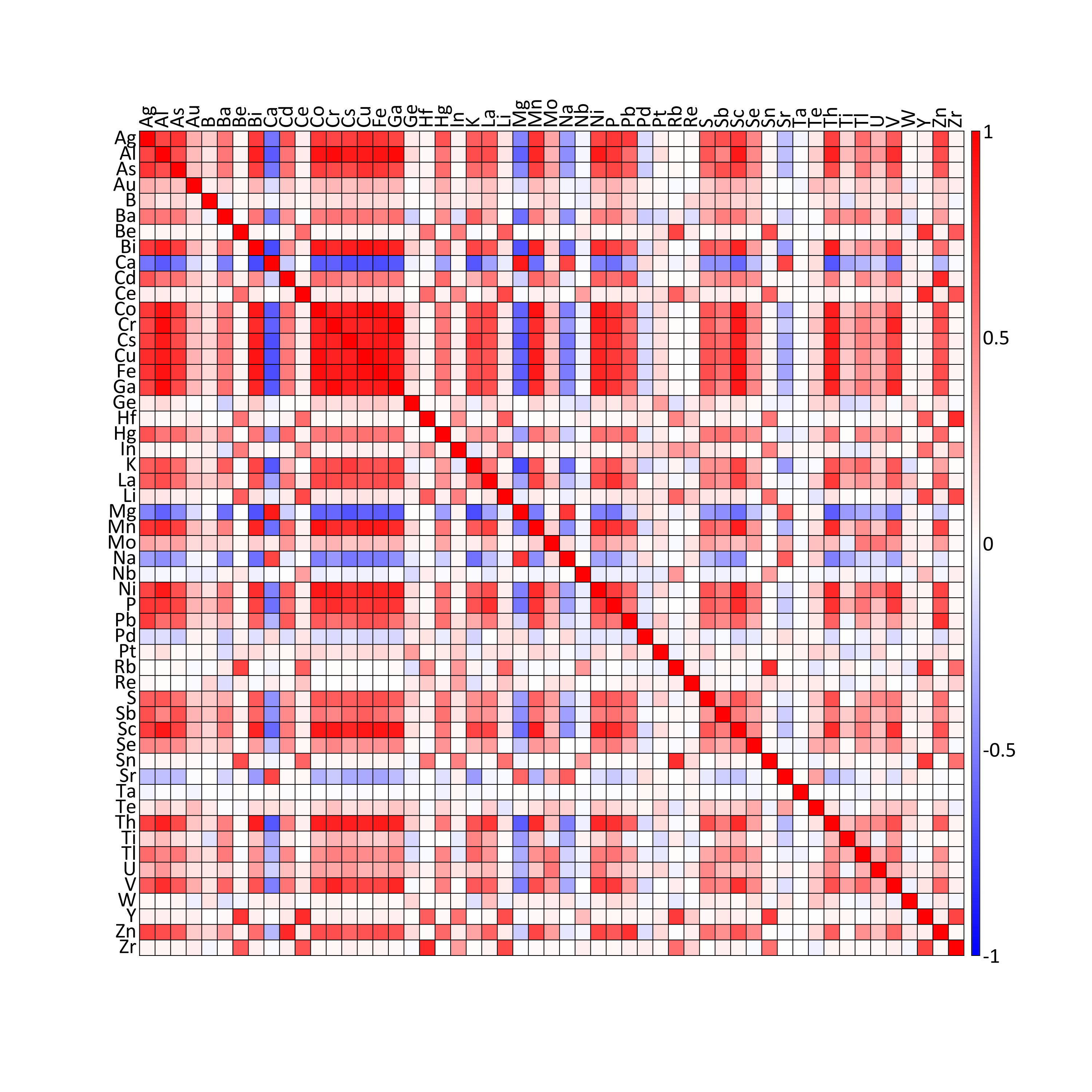
A geochemical dataset provides a more compelling example of PCA in terms of potential dimension reduction and exploratory analysis. This public data was collected by the Northwest Territories Geological Survey in partnership with the Geological Survey of Canada. It includes \(n=1660\) stream sediment samples that provide \(k=53\) elements, which were collected in mineral deposit exploration across the Mackenzie Mountains. After standardizing the elements, the covariance matrix of the resulting \(\mathbf{Y}\) data is calculated and displayed below.

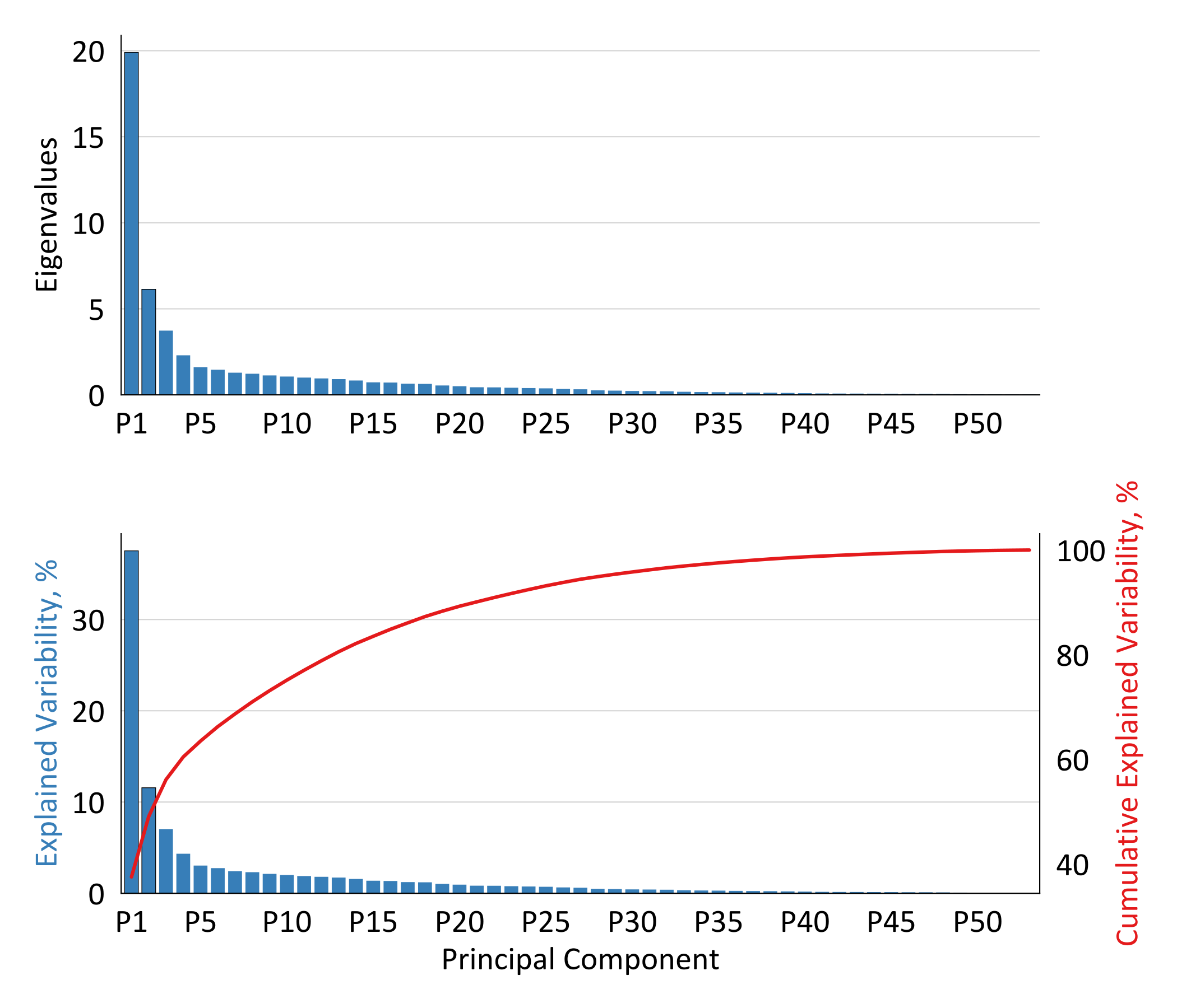
Spectral decomposition is applied to the covariance matrix, generating the eigenvalues displayed below. The explained variability of the principal components is then calculated from the eigenvalues, which is displayed in an incremental and cumulative manner. The cumulative plot is sometimes referred to as a scree or elbow plot. It is a useful tool, particularly if a visible elbow or inflection exists, where principal components begin explaining insignificant variability. A slight elbow exists here after the third or fourth component, though users may consider modeling additional components based on a required threshold of explained variability; say the 29 components that are required here to explain 95% of the variability.

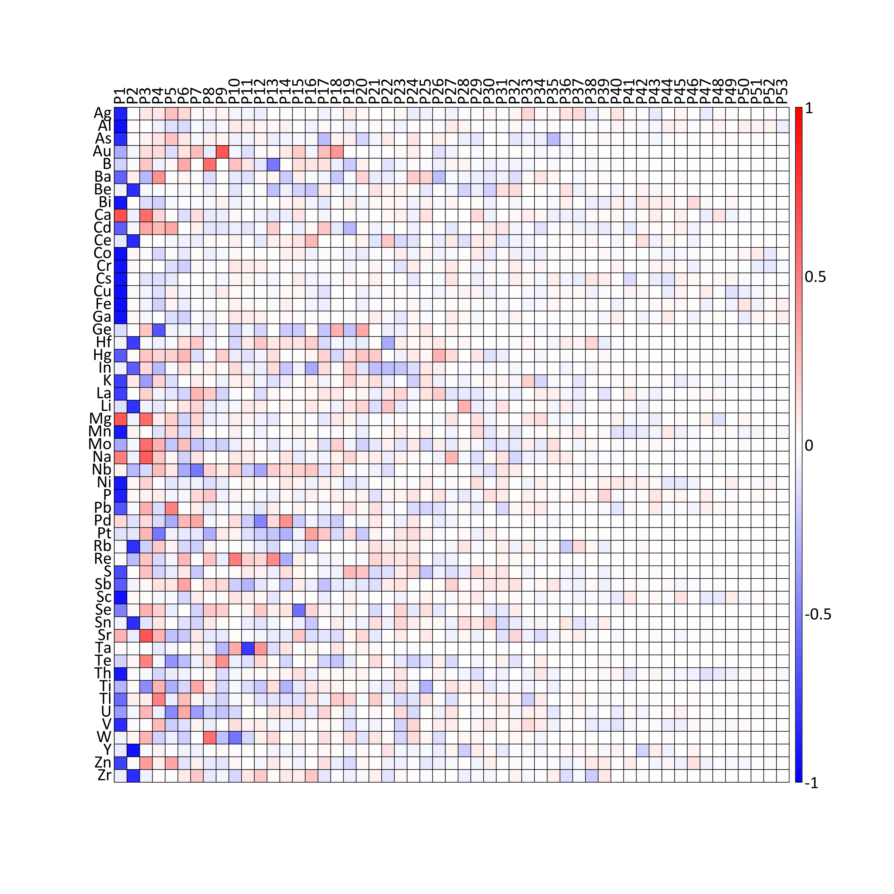
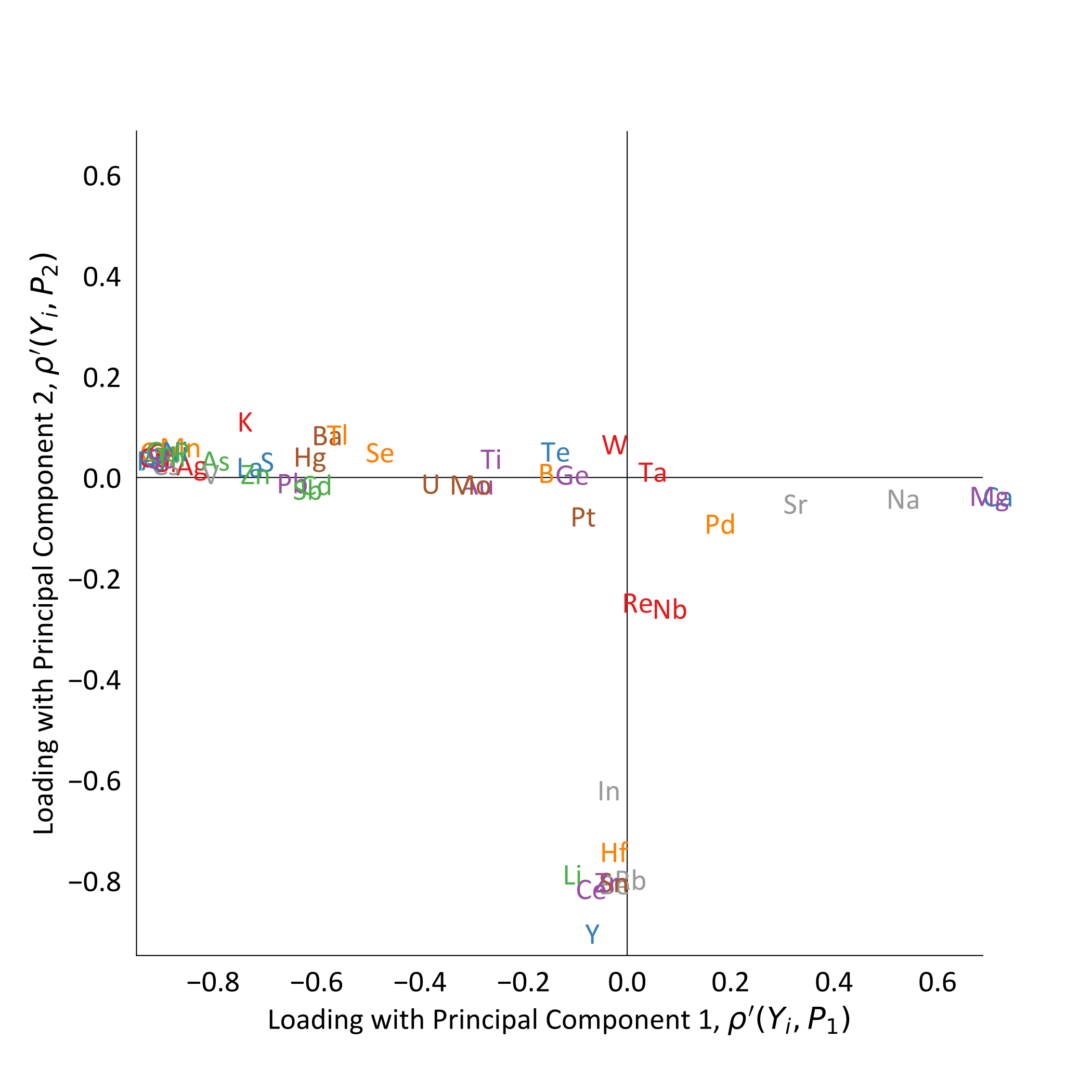
As expected based on the eigenvalues, most elements are only loaded strongly onto the first few principal components (matrix below). Consider that the volume of information in the covariance and loadings matricres above creates challenges for interpretting the overall multivariate system. A common exploratory analysis approach for simplifying the multivariate system and understanding the underlying latent variables, involves plotting the loadings of select principal components against each other, such as the first two principal components that are plotted below. Elements located in closely proximity are closely related, and vice versa. For example, consider that Ca and Mg have the largest P1 values (furthest right on the plot), while having very small P2 values. Their variability is largely explained by P1, but not P2. The two elements are located very near to each other and relatively far from other elements, which corresponds with the covariance matrix, where Ca and MgO are highly correlated with each other, and strongly negatively correlated with the most of the other elements. As only the first two principal component loadings are displayed, note that this is a simplified projection of the multivariate system, which only explains 49% of the variability.

Summary

PCA is a useful tool for multivariate geostatistical modeling. Geological variables are decorrelated to facilitate independent modeling, before the back-transform restores the original correlation to modeled variables. When the number of variables becomes impractical to model, the dimension reduction functionality of PCA may be used for modeling a subset of variables, before the back-transform provides models of all variables. It may also be applied for exploratory data analysis, providing insight into the underlying latent variables that explain a high dimensional multivariate system.

There are alternative linear decorrelation transformations that are immediate extensions of PCA, which may offer advantages to geostatistical modeling. These include data sphereing and minimum/maximum autocorrelation factors, which are the focus of a companion lesson.

References