Learning Objectives

• Identify the importance of a representative global distributions in estimation and simulation workflows
• Understand the principle of cell declustering
• Select parameters (especially the cell size) in cell declustering which will lead to a reasonable representative distribution

Introduction

Representative distributions and proportions are key input parameters to uncertainty assessment and simulation. Declustering techniques assign each datum a weight based on its closeness to surrounding data. All standard geostatistical texts include some discussion on declustering. The available data within a stationary domain \(z_i,i=1,\ldots,n\) are each assigned a weight \(w_i,i=1,\ldots,n\) based on the spatial proximity of the data. Data that are close get a reduced weight and data that are far apart get an increased weight. The premise being that closer data are more redundant and may preferentially sample low- or high-valued areas. A global non-parametric distribution or corrected categorical proportions are constructed using the weights and summary statistics also consider the weights. A representative distribution is useful for global resource assessment, checking estimated models and is required input to most simulation algorithms.

Polygonal declustering provides poor declustering weights except in relatively simple 2-D cases with very well understood lease or geological limits. Global estimation for declustering requires many parameters and can suffer from issues such as negative weights and high weights assigned to screened data. Considering a trend model for declustering can work; however, it only provides the corrected mean and many trend modeling algorithms require declustering weights as input. The technique of cell declustering is robust and widely used. This lesson addresses the selection of parameters for cell declustering.

Principle of Cell Declustering

Cell declustering was proposed by (Journel, 1983) and the first widely used public code was made available by the author (Deutsch, 1989). A version of that code (declus) is available in GSLIB (Deutsch & Journel, 1998). A grid of equal volume cells is placed over the domain. The cell size is unrelated to any cell or block size used in 3-D modeling; the cell size is approximately the spacing of the data in sparsely sampled regions. The number of occupied cells are counted (\(n_{occ}\)) and all occupied cells get the same weight. If there is only one data in a cell it gets a weight of \(1/n_{occ}\). If there are multiple data in the cell, then they share the weight assigned to the cell. The following figure illustrates this principle with eleven data and six occupied cells.

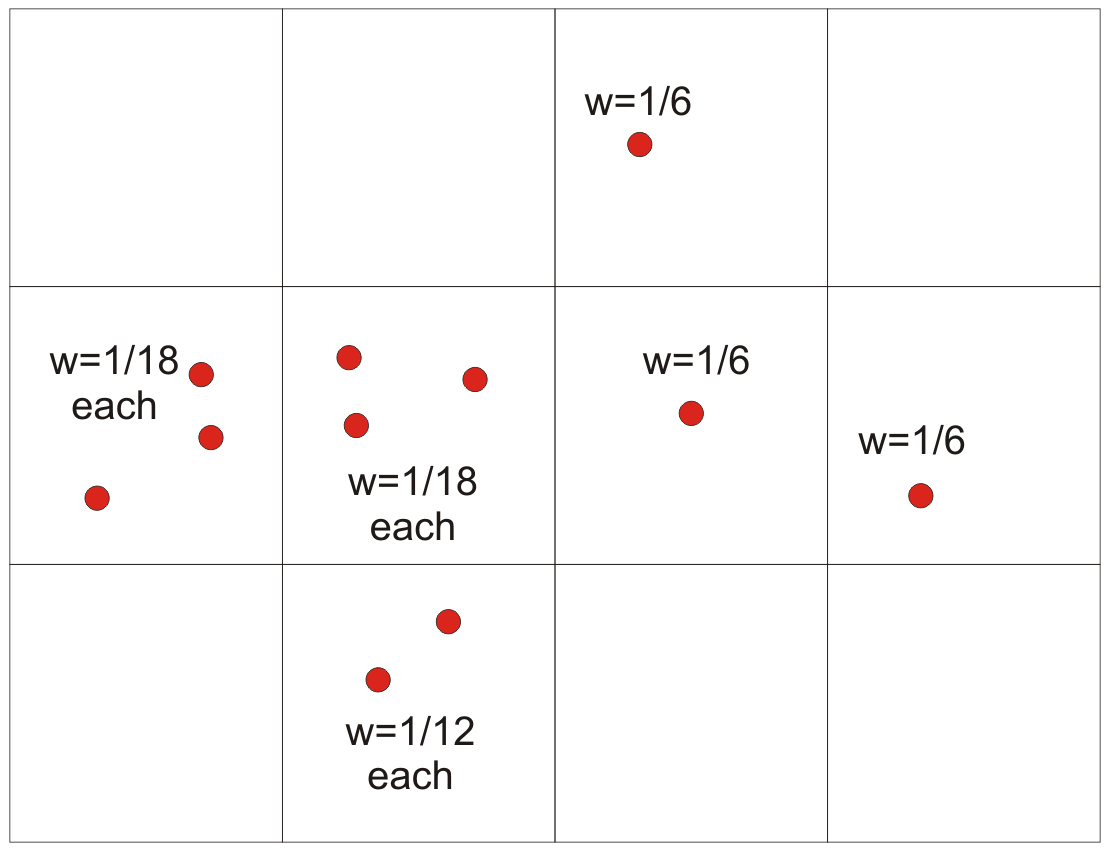
There are three obvious concerns and some more complex considerations in 3-D. First, any data that happens to fall on a cell boundary is randomly assigned to one cell. Second, the origin of the cell network changes the results and can lead to unstable results. The early declus program considered a limited number of origin offsets on a regular vector based on the cell size. The newer CellDeclus program considers a larger number of randomly chosen origins (as illustrated below with three origins). The weight to each data is an average of the weight coming from each origin. The third concern relates to the cell size.

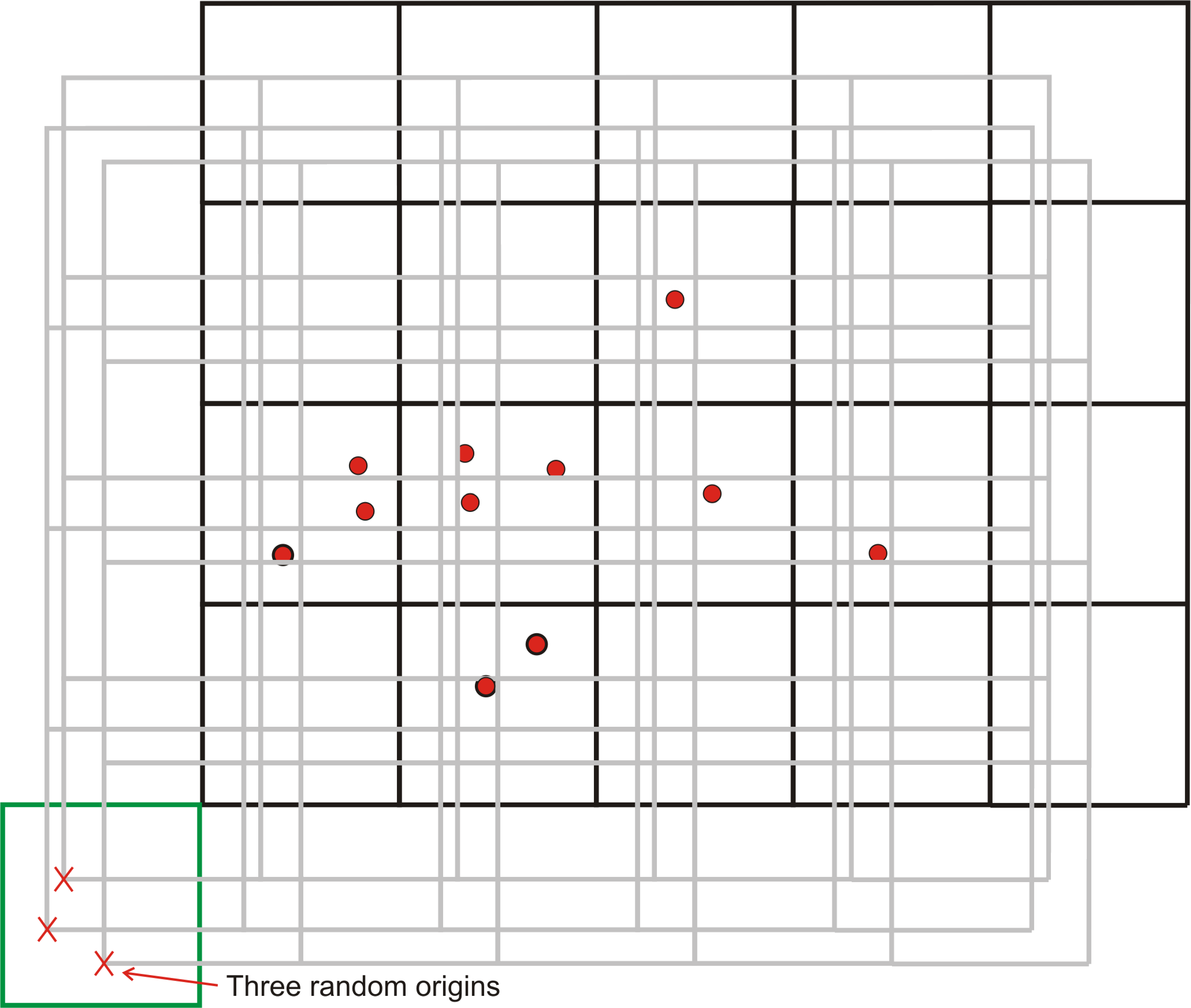
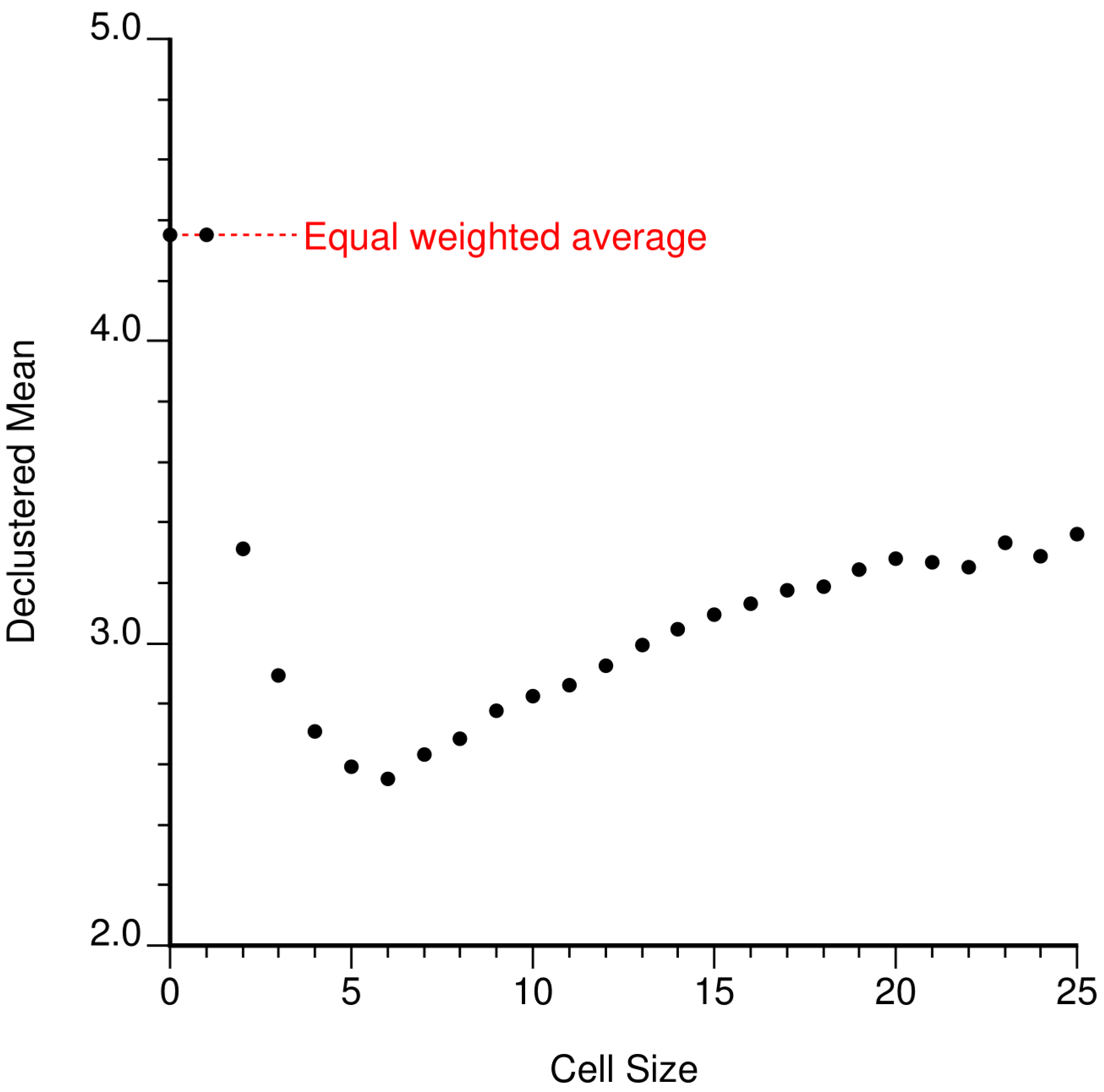
A very small cell size leads to many unoccupied cells and a single data in each occupied cell; the data are equally weighted. A very large cell size leads to nearly equal weighting because all data could fall into the same cell. Regardless of how large the cell size, randomizing the origin will split the data into as many as four cells in 2-D and eight cells in 3-D. The data are not equally weighted with large cell sizes. Considering the range from small cell size to large cell size led to the popularization of a diagnostic plot of declustered mean versus cell size. An example is shown below. Note that (1) the first two cell sizes lead to the same result because no data are closer than one distance unit, (2) the declustered mean for large cell sizes does not increase to the equal weighted mean, and (3) this plot shows a clear minimum that corresponds to the size of data clusters (this is the data provided with the GSLIB book (Deutsch & Journel, 1998)). There is no theoretical expectation that the minimum or maximum is correct, but this plot is widely viewed to help with parameter selection. In practice, choosing the parameters for cell declustering may be more complex.

Parameter Selection

The following reviews the parameter choices involved in cell declustering. It is common to decluster data within each stationary domain separately. This can sometimes lead to edge effects or overweighting when the domain pinches out, but it is difficult to consider any other approach. It is also common to use the same declustering weights for multiple variables provided the variables are equally sampled, that is, all available at all data locations. If the data are unequally sampled, then debiasing and data imputation should be considered.

2-D versus 3-D

All geological formations are 3-D, but there are many cases when 2-D declustering is appropriate. Sometimes the variables are averaged across the full thickness of the deposit and 2-D declustering is correct. Delineation drilling in a tabular or stratabound deposit is often perpendicular to the plane of greatest continuity and the dilling fully intersects the zone of interest. Declustering in 2-D, that is, the plane of continuity is appropriate since there is no clustering in the third dimension. 2-D declustering is always preferable since there is less risk of some unexpected weighting to occur. There are situations with highly deviated drilling that require a 3-D declustering. The presence of long horizontal wells with many data in a petroleum reservoir context are problematic; one recommended approach is to leave the horizontal data out of declustering and distribution inference. The data would be included as conditioning data in subsequent facies and property modeling.

Coordinate System

The coordinates used in declustering should align with the principle directions of sampling. The two cell declustering programs mentioned above consider that the input X, Y and Z coordinates are the principle directions. A prior rotation may be applied. A flattening or unfolding may also be applied in stratabound cases. The input data to cell declustering consists of locations in a reasonable X, Y and Z coordinate system with the most important variable specified for creating the diagnostic plot and checking the results.

Anisotropy

No anisotropy specification is required in the case of a disseminated nearly isotropic geological environment. No anisotropy specification is likely required in the case of 2-D declustering. The anisotropy of cell declustering should approximately follow the anisotropy of sampling which, in turn, usually follows the anisotropy of the geological formation. An anisotropy of 0.25% to 1% (0.0025 to 0.01) may be required in stratigraphic deposits. Most cell declustering software allows a ratio to be specified for Y to X (normally 1) and for Z to X (normally less than 1, say 0.01 for stratigraphic cases). This ratio is applied to all cell sizes being considered. As different X cell sizes are considered, then the Y and Z cell sizes are set with the specified anisotropy ratio. The user can always rerun cell declustering with different anisotropy ratios if there is doubt. This will permit an understanding of sensitivity, but will not likely resolve any ambiguity. In practice, the choice of the optimal X cell size is more important than the anisotropy specification.

Range of Cell Sizes

A range of cell sizes is chosen to plot the diagnostic plot shown above and to assist in the selection of an optimal cell size. The result for a zero cell size is the equal weighted value. A too-small minimum cell size should not be chosen because the number of cells would get too large. The old declus program allocated an array the size of the grid, which was very inefficient. The newer CellDeclus program simply keeps the grid index associated to each data, but the number of cells still cannot be too big since the index could overflow numerical precision. In practice, the minimum cell size could be set to the closest practical spacing of the data

The “correct” cell size is the spacing of the data in the sparsely sampled areas. This correct size is not exactly known and a range of cell sizes is considered to provide some help selecting the right answer. So, the maximum cell size should not be set too large. It is not like the variogram that could have a range larger than the spacing of the data. The maximum should be less than one half of the domain size. The size is relative to the X extent of the domain; the Y and Z extent will be determined by the specified anisotropy.

The number of cells between the minimum and maximum should be enough to see the character of the declustering plot. Normally between 25 and 100 different cell sizes works well. If the minimum is reasonable (not too small), then the number of cells could be chosen as a multiple of the minimum size, that is, (max - min)/min. For example, given a domain 10000 units large in X with a chosen minimum of 100 units, we could take the maximum to be 4000 units and (4000-100)/100=39 cells. This will give us 39 evenly spaced cell sizes 100, 200, 300,…,4000. It is not essential to have this even spacing.

Optimal Cell Size

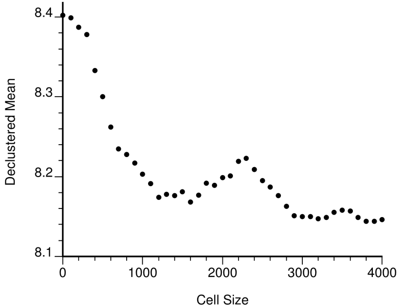
The most challenging decision is how to choose an optimal cell size in the principal X direction (the anisotropy is already accounted for). Choosing the spacing in the sparsely sampled areas is reasonable when there is an underlying regular grid of data spacing followed by some areas more closely drilled; however, the drilling is often irregular. Choosing the optimal cell size based on the diagnostic plot may also be difficult. The plot shown above is straightforward with one clear minima that makes sense. The plot below is unclear. There is a plateau between 1200 to 1600 distance units, then there is another between 3000 and 4000 distance units. In this case, knowing the data configuration, we would want to take a value of around 1200 distance units. It is common that the first minima/plateau is the correct one. Additional support is sometimes required.

When there is no obvious reasonable size and no clear indication on the diagnostic plot, a high resolution data spacing model is useful to help choose the cell size. There are many different programs and algorithms to compute data spacing. This is not the subject here. Computing the data spacing on a high resolution grid and plotting the results as a cumulative distribution can be helpful. The following shows a CDF of data spacing the lower tail is in areas of clustered samples. The steep region is where the data spacing is nearly constant. The upper tail is where the data spacing is increasing near the borders of the study area.

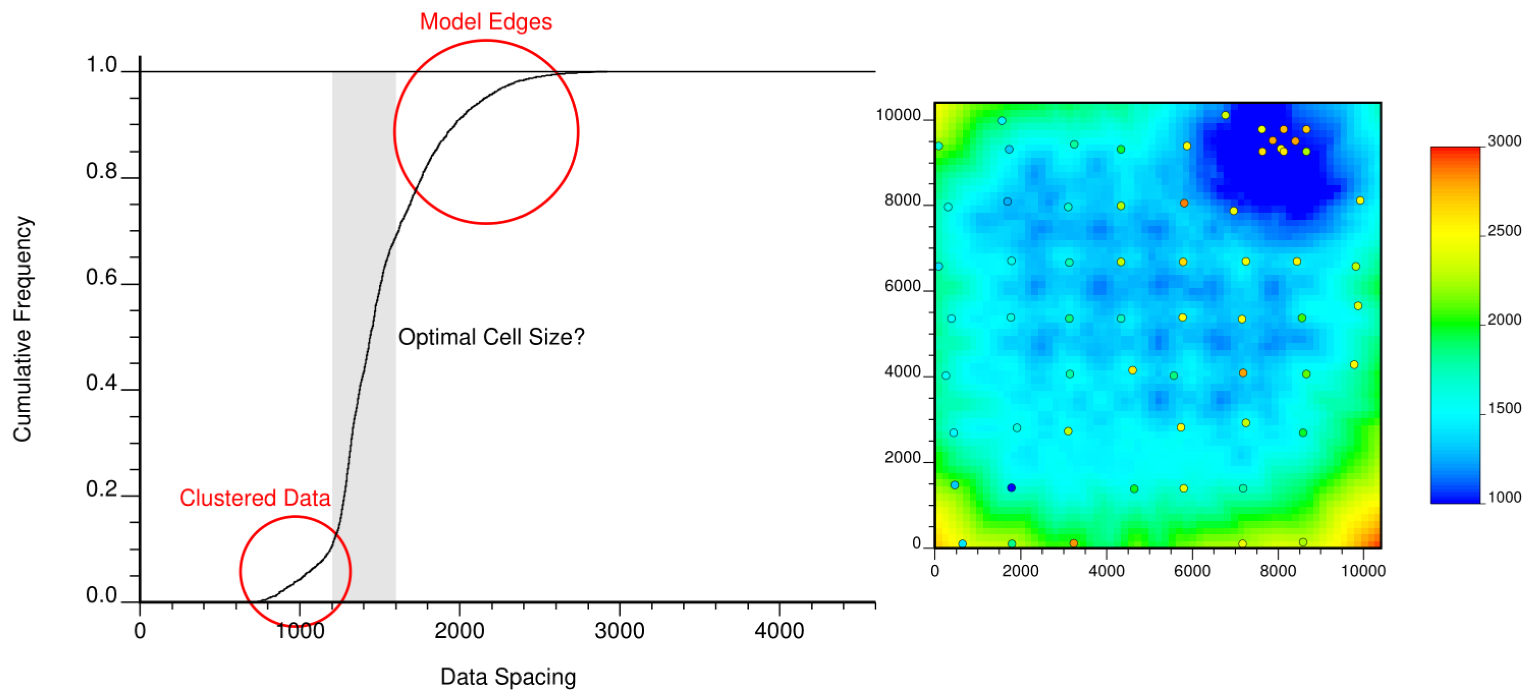
There is no “optimal” cell size in the sense of a clearly defined objective function, but the cell size retained for the final distribution should (1) be a reasonable size relative to the spacing of the sparsely sampled data, (2) show a near minimum or a plateau on the cell declustering diagnostic plot, and (3) seem like a reasonable data spacing on the distribution of data spacing.

Summary

Declustering remains an underappreciated step in geostatistical modeling. In practice, a global representative distribution of every continuous and categorical variable is essential for unbiased resources/reserves calculation and the accurate and precise representation of uncertainty. Cell declustering is a widely used technique and this lesson reviews some details of parameter selection.

References