Learning Objectives

• Define the multivariate Gaussian distribution
• Understand essential properties of the multivariate Gaussian distribution
• Review the importance of the multivariate Gaussian distribution to geostatistics

Introduction

One of the core challenges in geostatistics is to represent the multi-dimensional distribution of multiple variables at many locations given the few sample data available. In most circumstances, less than a billionth of a deposit is extracted for sampling before development decisions are taken (Pyrcz & Deutsch, 2014). Predicting conditional distributions of uncertainty at unsampled locations requires a multivariate distribution between the unsampled location and available sample data within a search distance. It is not possible to define these multivariate distributions non parametrically due to the unique configuration of locations for each unsampled location. The parametric multivariate Gaussian (MG) distribution is widely adopted.

The MG distribution is unique for being mathematically manageable; it is fully parameterized by a mean vector and a variance-covariance matrix. In geostatistics the variance-covariance matrix is derived from variogram models, while the mean vector comes from an assumption of stationarity within the geological domain (Pyrcz & Deutsch, 2018). The MG distribution permits straightforward inference of conditional distributions; therefore, many geostatistical algorithms and software take advantage of the MG distribution to predict the conditional distributions of continuous geological variables (Deutsch, 2020).

Although geological properties are not naturally Gaussian distributed, the transformation to a univariate Gaussian distribution is common practice in geostatistics, see Normal Score Transformation Lesson (Pyrcz & Deutsch, 2018). In the context of geostatistics, calculations are performed in a stationary domain \(A\) that belongs together geologically. A multivariate spatial Gaussian distribution is assumed for all locations in the domain after univariate transformation. The conditional distribution (\(f\)) of a random variable \(Z\) at an unsampled location \(\mathbf{u}\) conditioned to the available data \(n\) is denoted:

\[f_{z(\mathbf{u})|n}(z), \forall \:\: \mathbf{u} \in A\]

This is defined by multivariate distributions:

\[f_{z(\mathbf{u})|n}(z) = \frac{f_{z(\mathbf{u}),Z_1,...,Z_n}(z(\mathbf{u}),z_1,...,z_n)}{f_{Z_1,...,Z_n}(z_1,...,z_n)}\]

The distribution at an unsampled location is the \(n+1\) variate (data + unsampled location) distribution divided by the \(n\) variate (data) distribution. These relatively high-dimensional distributions cannot be directly predicted non-parametrically due to a lack of repetitive sample configurations. The MG distribution provides a practical approach for spatially correlated variables.

This lesson will review the definition of the MG distribution, some essential properties, and its importance and application in geostatistics.

Multivariate Gaussian Distribution - Definition

The MG distribution is a generalization of the univariate Gaussian to higher dimensions (Johnson, Wichern, et al., 2014). The univariate Gaussian distribution for a random variable \(Y\) with mean \(\mu\) and variance \(\sigma^2\) is represented by:

\[f(y) = \frac{1}{{ \sqrt {2\pi\sigma^2 } }}e^{{{ -[ \left( {y - \mu }\right)/\sigma]^2/2 }}}\]

The MG distribution has its probability density function represented as:

\[ f\left( \mathbf{y}; \boldsymbol\mu , \mathbf{\Sigma} \right) = \frac{1}{\left( \sqrt{2 \pi} \right)^d | \mathbf{\Sigma} |^{1/2}} e ^\frac{-(\mathbf{y}-\boldsymbol\mu)^T \mathbf{\Sigma}^{-1}(\mathbf{y}-\boldsymbol\mu) }{2} \]

The exponent of the univariate function represents the squared distance from \(y\) to \(\mu\). For the multivariate, \(\mathbf{y}\) is a vector that represents position in an \(n\) dimensional space.

\[\begin{align} \mathbf{y} &= \begin{bmatrix} y_{1} \\ y_{2} \\ \vdots \\ y_{n} \end{bmatrix} \end{align}\]

\(\boldsymbol\mu\) is the mean vector, that is, the expected value in every dimension:

\[\begin{align} \boldsymbol\mu &= \begin{bmatrix} \mu_{1} \\ \mu_{2} \\ \vdots \\ \mu_{n} \end{bmatrix} \end{align}\]

\(\mathbf{\Sigma}\) is the variance (\(\sigma^2\))-covariance (\(C\)) matrix for all pairs:

\[\begin{align} \mathbf{\Sigma} &= \begin{bmatrix} {\sigma^2}_1 & C_{1,2} & \cdots & C_{1,n}\\ C_{2,1} & {\sigma^2}_2 & \cdots & C_{2,n}\\ \vdots & \vdots & \ddots & \vdots\\ C_{n,1} & C_{n,2} & \cdots & {\sigma^2}_n \end{bmatrix} \end{align}\]

The variance-covariance matrix \(\mathbf{\Sigma}\) must be positive definite. \(|\mathbf{\Sigma}|\) is the determinant of the variance-covariance matrix, and \(\mathbf{\Sigma}^{-1}\) is the inverse.

The generating mechanism of the Gaussian distribution is the central limit theorem. The central limit theorem states that the distribution of the sum of many independent samples of a random variable (RV) with finite mean and variance tends to a Gaussian distribution as the number of samples increases. The characteristic bell shape of the univariate Gaussian distribution and the characteristic ellipsoidal contours of the bivariate distribution are well known, see the figure.

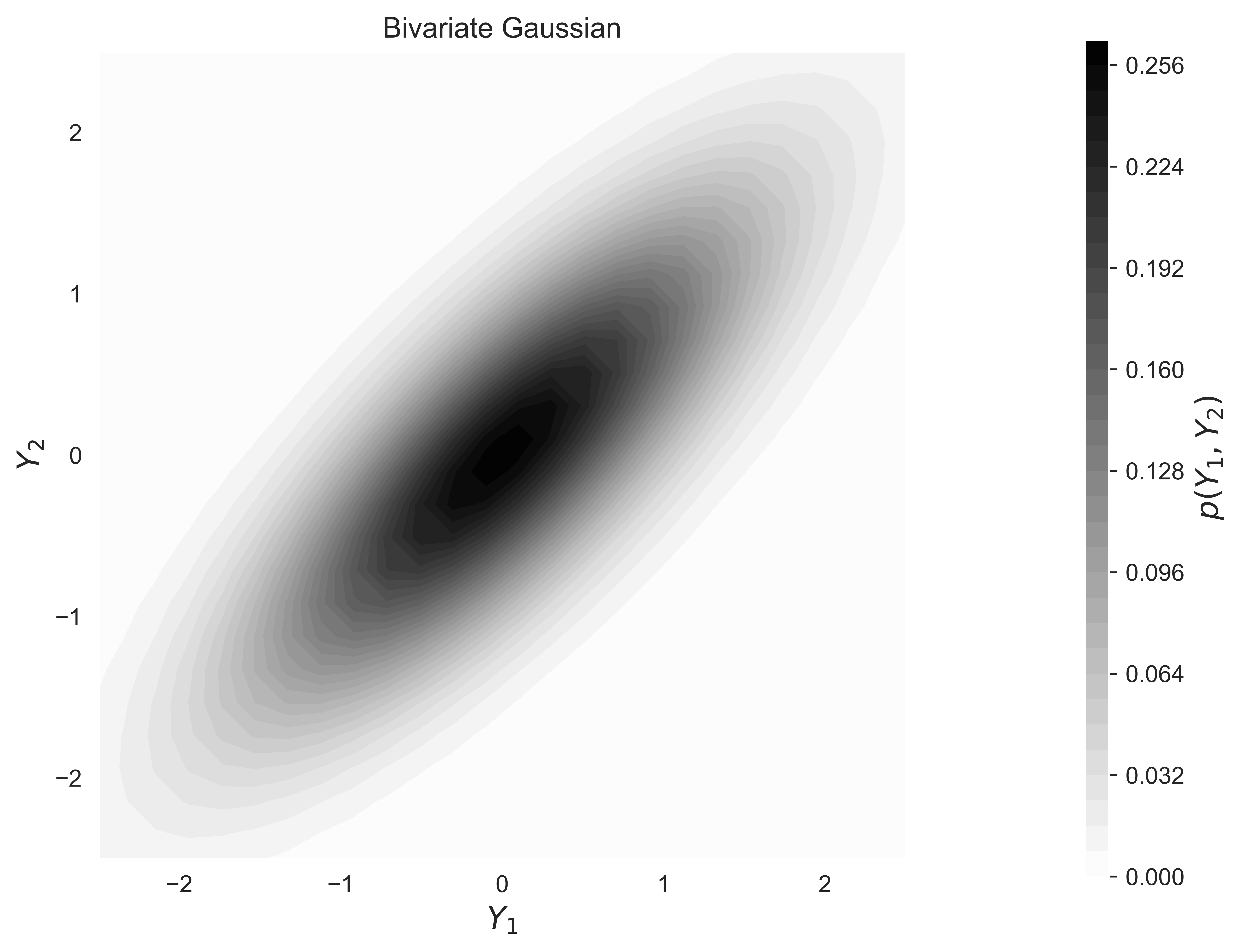
The MG distribution is fully defined by the mean vector and the variance-covariance matrix. This straightforward parameterization and its properties make the MG distribution the most important distribution in geostatistics (Barnett & Deutsch, 2011).

Multivariate Gaussian Distribution Properties

There are four main properties of the MG distribution that geostatistical algorithms rely on.

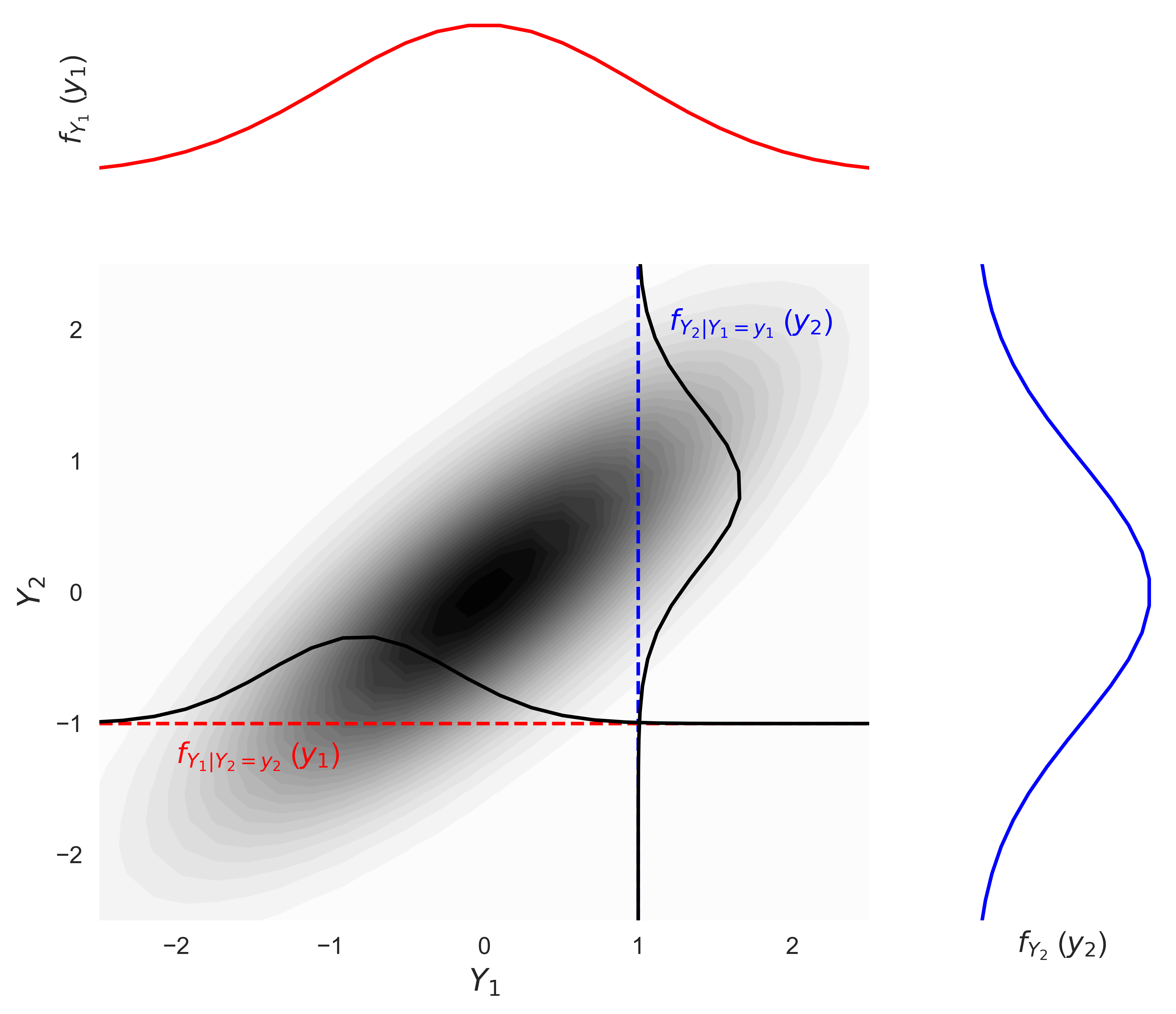
1. All lower order distributions of the MG distribution, such as conditional and marginal distributions, are Gaussian.

The figure below shows an example of a bivariate Gaussian distribution of variables \(Y_1\) and \(Y_2\), and their respective marginal distribution that are also Gaussian. The figure also illustrates conditional distributions following a Gaussian shape.

2. All conditional expectations are linear function of the data.

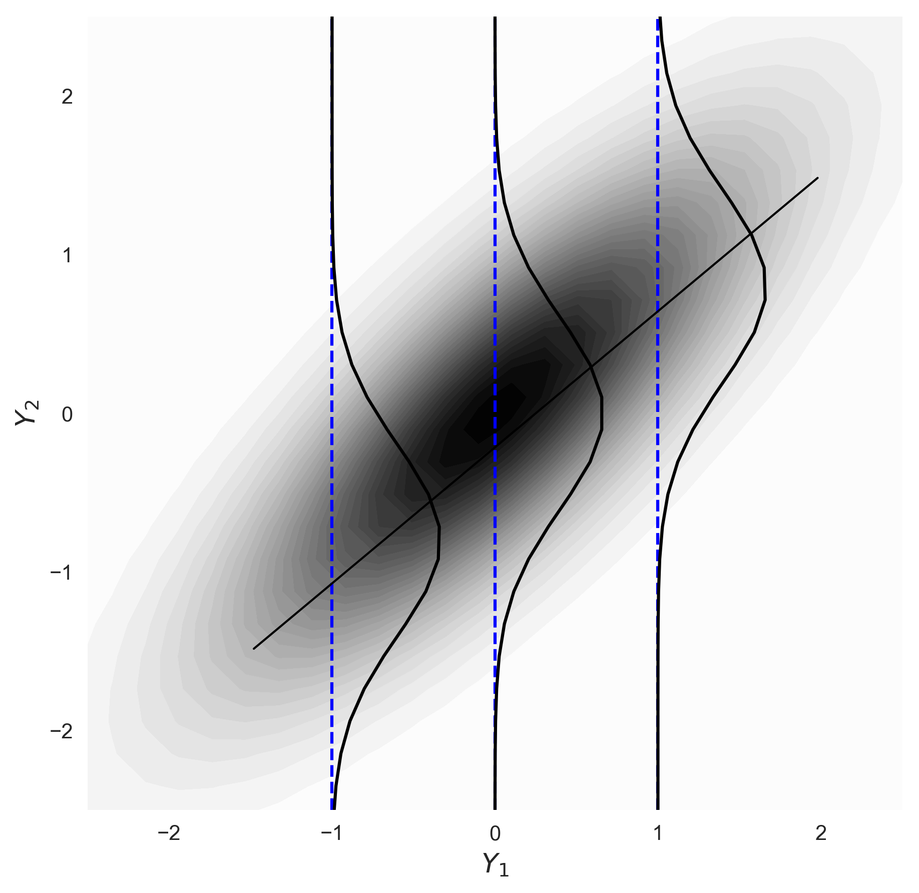
This is also illustrated on the next figure. Linear regression is theoretically correct in the presence of MG distributed variables. Consider standard Gaussian variables that come from the normal score transform (detailed in an accompanying Lesson) or standardizing a non-standard Gaussian variable:

\[ Y = \frac{Z-\mu}{\sigma} \]

The mean (\(\mu\)) and standard deviation (\(\sigma\)) to \(y\) are \(\mu = 0\) and \(\sigma = 1\).

Consider a bivariate case with standardized random variables \(Y_1\) and \(Y_2\), the conditional expectation of \(Y_2\) given \(Y_1 = y_1\) is:

\[E(Y_2|Y_1=y_1) = \rho y_1\]

that is, a linear function of \(y_1\).

3. All conditional variances are data value independent.

Considering standard values again, the conditional variance is given by

\[ var(Y_2|Y_1=y_1) = 1 -\rho^2\]

that is, the conditional variance does not depend on the conditioning value \(y_1\).

4. The conditional distributions are defined by the normal equations.

Consider all data values and the unsampled locations following an MG distribution. Let \(y_0\) be the variable to be predicted and \(y_1, ..., y_n\) be condtioning data. They are indexed by specific locations. The distribution \(f_{y_0|n}(y)\) is Gaussian with a conditional mean that is a linear function of the conditioning data:

\[\mu_c= \sum_{\alpha=1}^{n} \lambda_\alpha y_\alpha\]

and a conditional variance that does not depend on the data values:

\[{\sigma^2}_c= {\sigma}^2 - \sum_{\alpha=1}^n \lambda_\alpha C_{\alpha 0}\]

where all \(C\) (covariance) values are inferred from the variogram of the normal scores (\(C=1-\gamma\)). The linear weights (\(\lambda_\alpha , \alpha=1,\ldots,n\)) come from the normal equations:

\[ \sum_{\beta=1}^n \lambda_\beta C_{\alpha \beta} = C_{\alpha 0} \:\: , \:\: \alpha=1, \ldots ,n\]

clarifying that the normal equations define the conditional distributions. In geostatistics, the normal equations are known as Simple Kriging (SK).

Geostatistics Application

Due to the properties described above, the MG distribution is extensively used in geostatistical algorithms. At the time of this Lesson, there is no other known distribution that can be used for inference in a high dimensional multilocation and multivariate situation. A commonly encountered case in geostatistics considers one variable and multiple locations. This is the multiGaussian kriging approach (PostMG) (Verly, 1983) summarized as:

1. A global representative distribution is inferred for the deemed stationary domain using declustering if necessary. Data are transformed to normal scores and the transformation table containing the original values and corresponding normal scores is kept.

2. The variogram of the normal score data is calculated, interpreted, and modeled. The model provides the covariances necessary to fully parameterize the MG distribution for the domain.

3. The normal equations (simple kriging) is performed at each unsampled location to calculate the local mean and variance. These local mean and variance values define the local conditional Gaussian distributions.

4. A reasonably large number \(L\), e.g. \(L=200\), of quantiles are defined to back transform each local distribution to original values: \[ p_l = \frac{l}{L+1}, \;\; l=1,\ldots, L \] \[ z_l({\mathbf{u}})= F^{-1} \left( G \left( G^{-1}(p_l) \cdot \sigma_c({\mathbf{u}})+m_c({\mathbf{u}}) \right) \right), \;\; l=1,\ldots L,\;\; \forall \;\; {\mathbf{u}} \]

where \(G^{-1}\) is the inverse of the standard normal CDF. The local conditional mean and standard deviation values are denoted \(m_c({\mathbf{u}})\) and \(\sigma_c({\mathbf{u}})\). All conditional distributions are back transformed. The expected value in original units and summary measures of local uncertainty could be inferred including the probability of exceeding a critical threshold (Pinto, 2020). Note that the distributions established by the MG kriging workflow are at the scale of the data and simulation is required to consider block or large scale uncertainty.

MultiGaussian Kriging Example

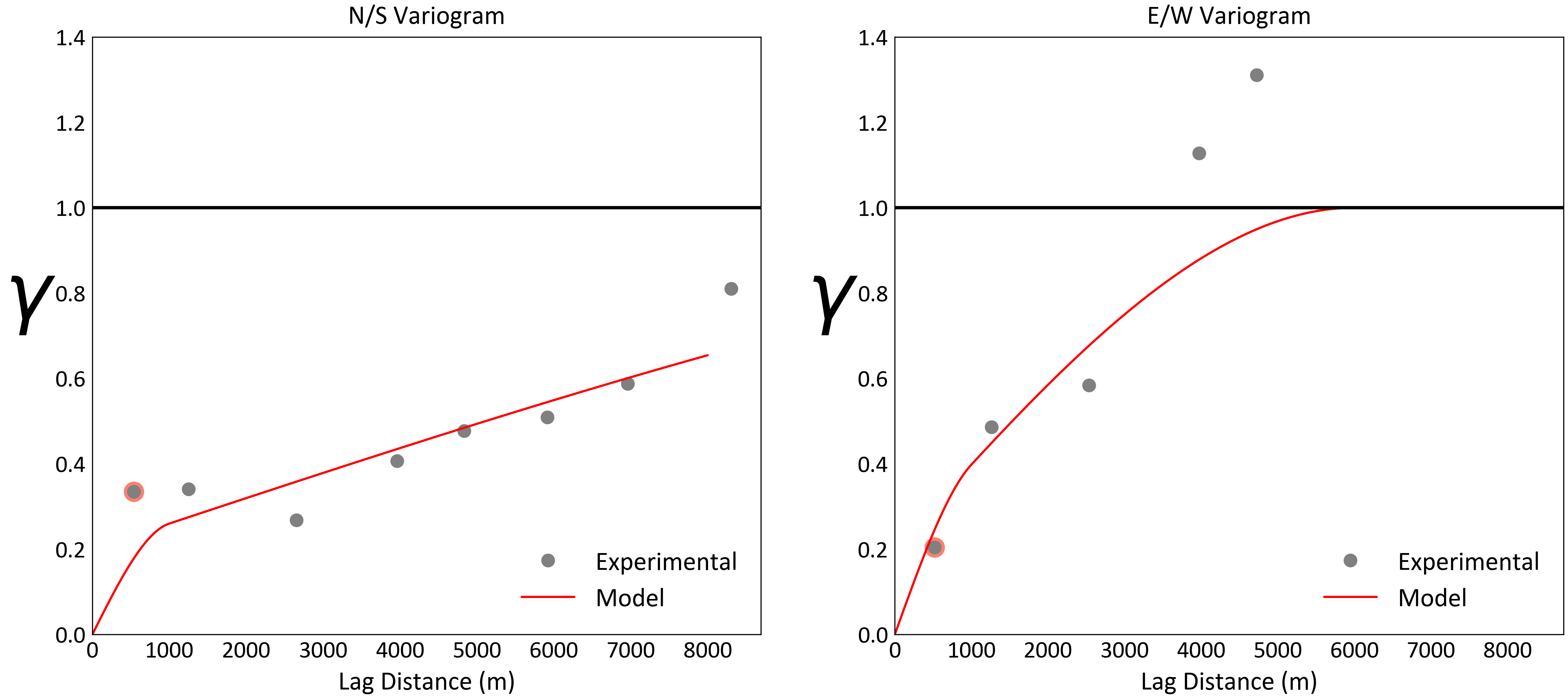
A brief example using the ConklinWell2D porosity data demonstrates this workflow. A location map and directional variograms are shown below.

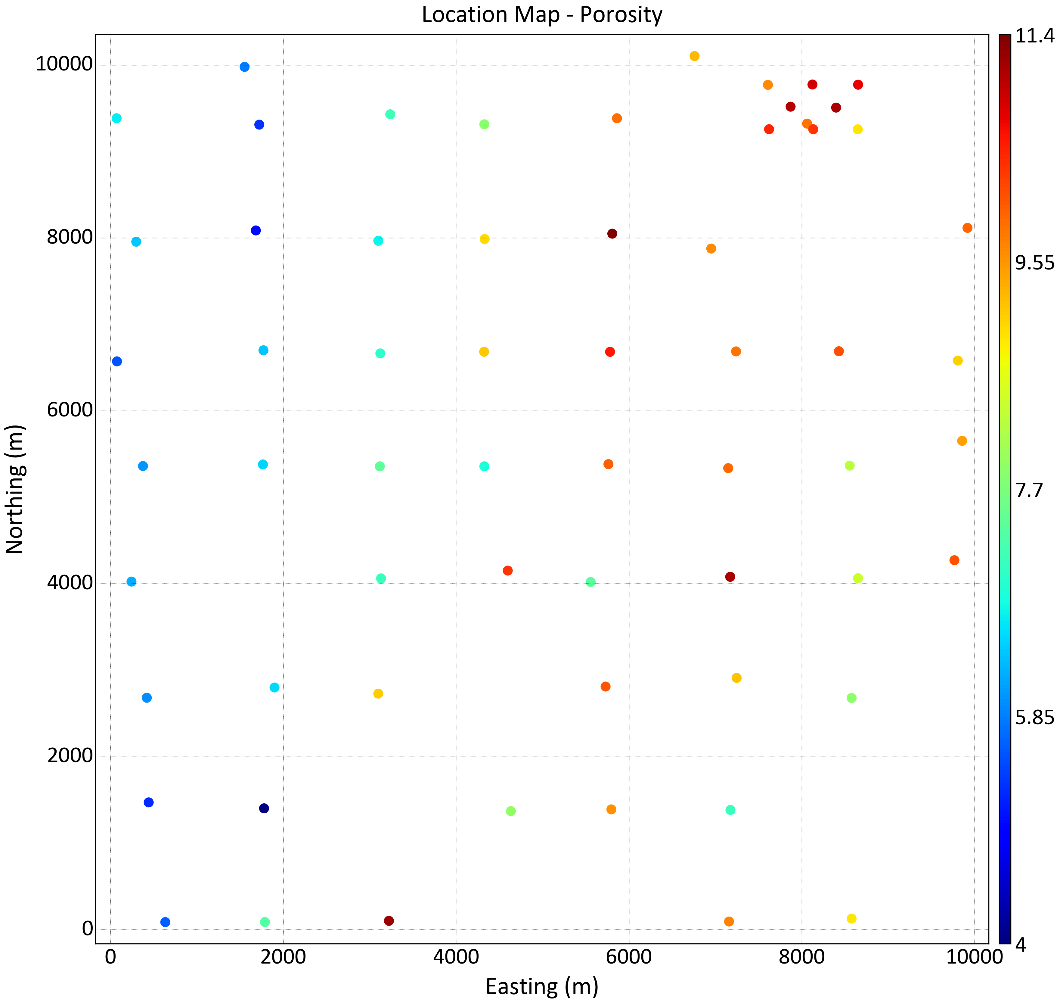
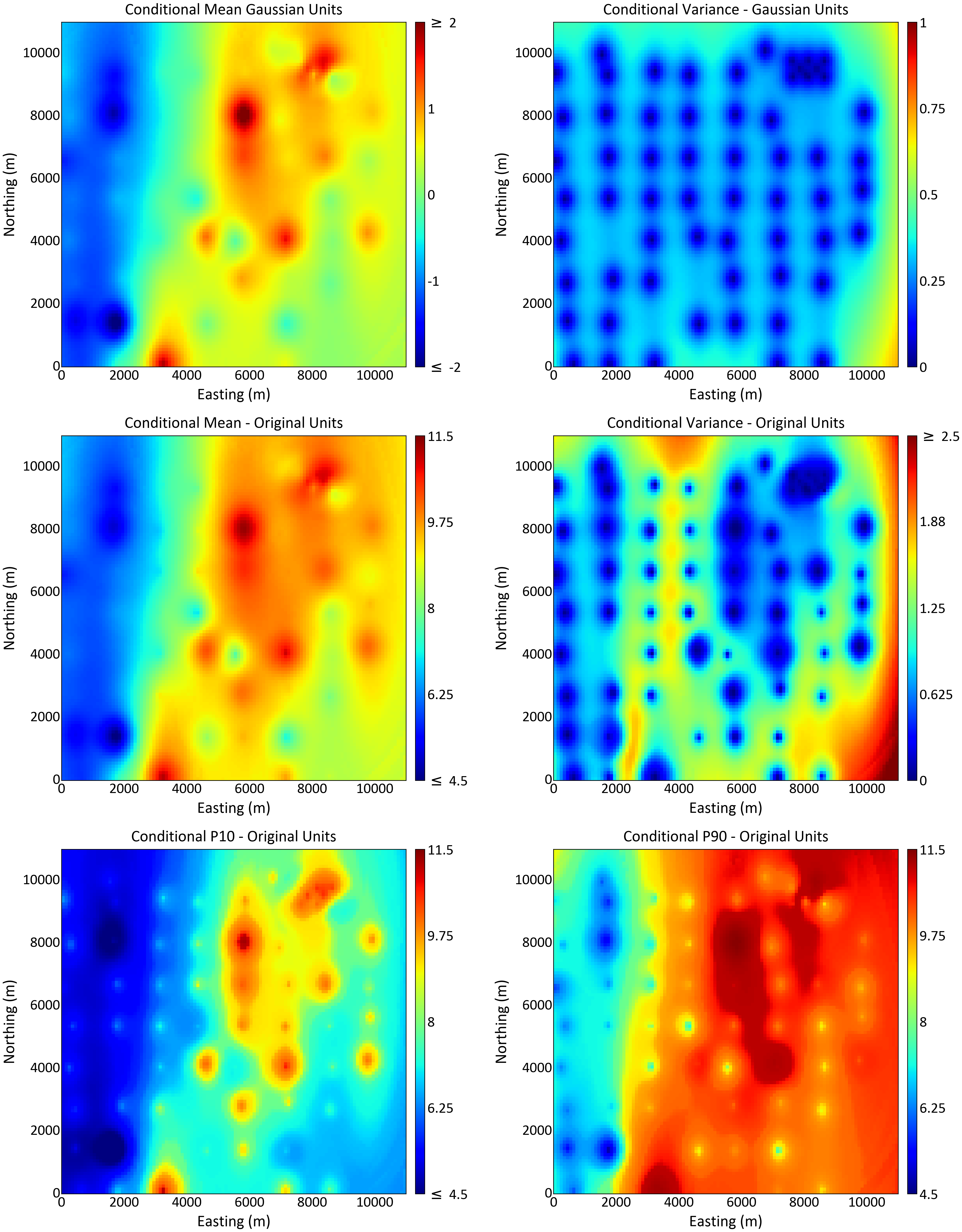
The conditional mean and variance in Gaussian units are calculated by simple kriging (top row). The PostMG back transform is executed and the conditional mean and variance in original units is obtained and shown on the second row. Note how the back transformed variance depends on the data values; in particular, note the band of high uncertainty separating the low and high values. The conditional P10 give us 90% chance of being higher than a specific value; where this value is high we are surely high. The conditional P90 indicates 10% chance of being higher (90% chance of being lower); where this value is low we are surely low.

As mentioned above, the uncertainty of blocks or at any larger scale requires simulation (Ortiz, Leuangthong, & Deutsch, 2004). Sequential Gaussian simulation is one implementation of many that could be considered.

Sequential Gaussian Simulation

Simulated realizations are used when we require measures of uncertainty that involve multiple locations. Simulation generates realizations that reproduce the data, the input histogram and the input variogram within statistical fluctuations (Pinto, 2020). Sequential Gaussian Simulation (SGS) depends on a recursive application of the definition of a conditional distribution to define the joint distribution of \(N\) RVs. \(N\) represents the number of simulation locations and is usually large, for example, millions of locations are considered to discretize a geological site. SGS follows:

1. A random path is defined, each node is visited once
2. Search for nearby conditioning data and previously simulated values and solve the normal equations to calculate conditional mean and variance for the location
3. Draw a value simulated from the distribution and add it to conditioning data
4. Move to next node

Multiple realizations are simulated with different random numbers that are used to define the random path and the simulated values.

SGS Example

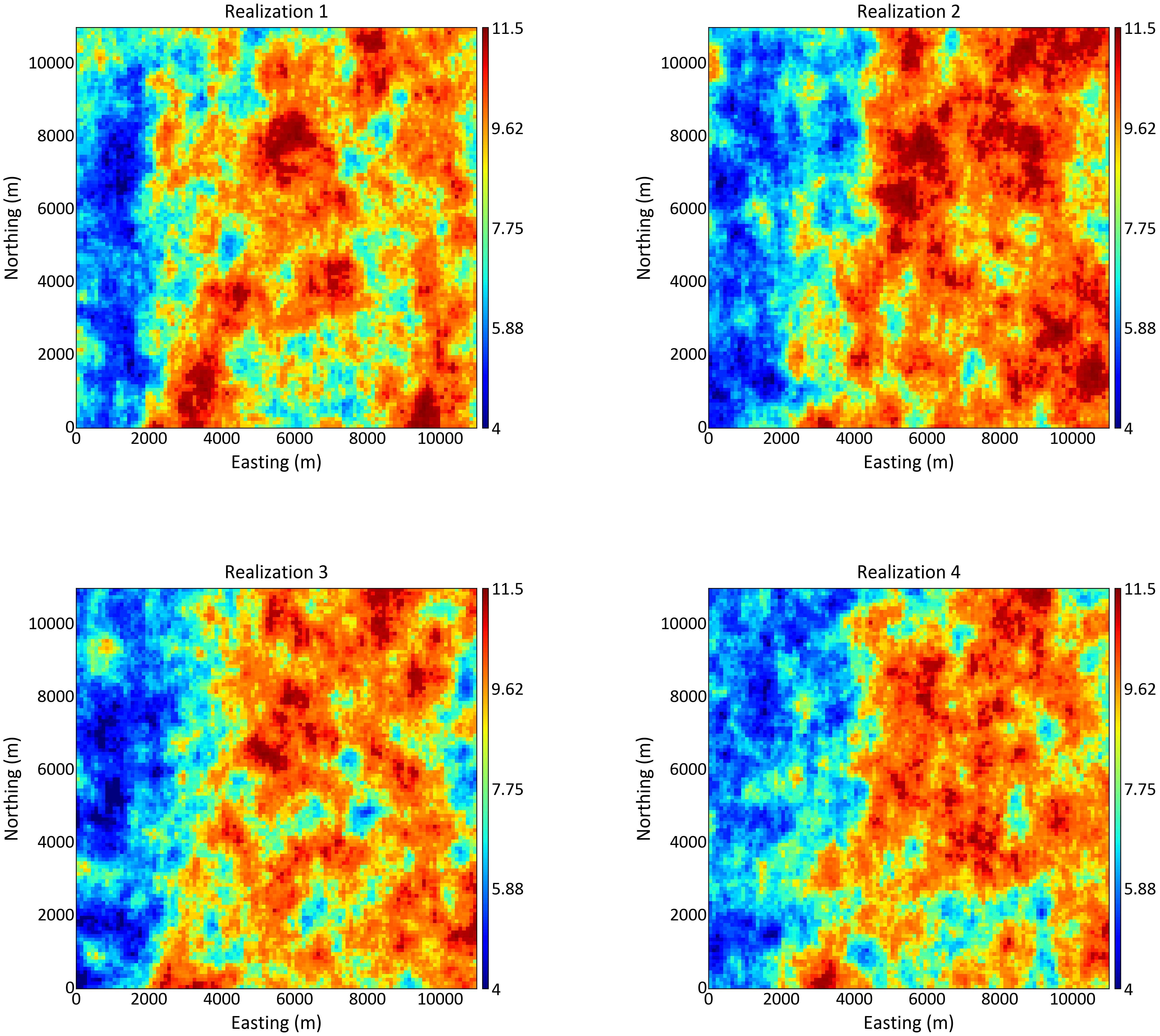
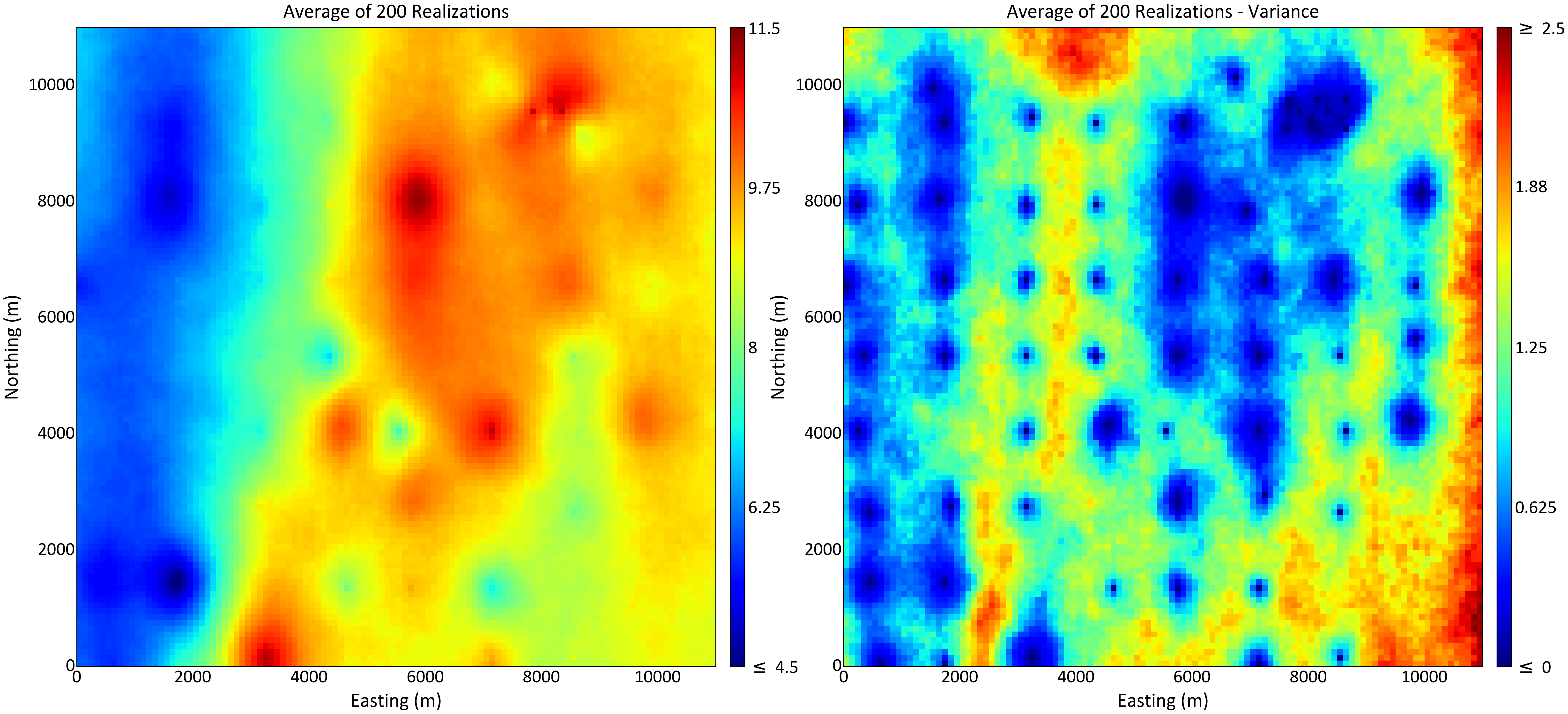
The first 4 of 200 SGS realizations are shown in the following figure. The average of all 200 realizations of SGS is shown in the figure below. The average reproduces the results of direct back transform shown above. The MG estimation framework provides local uncertainty, but it does not give a measure of joint spatial uncertainty of the variable at multiple locations. Simulation provides access to multiple location spatial uncertainty.

Multiple Variables

In theory, the extension to multiple variables is straightforward. A positive definite model of covariance between all locations and all variables is constructed and calculations proceed as described above. The positive definite covariance model is through the linear model of coregionalization (LMC). The LMC allows simple cokriging to be used in place of simple kriging and conditional distributions to be calculated in presence of multiple variables. Fitting an LMC from sparse data, however, is considered difficult in practice and alternatives are considered. One alternative is to assume some form of intrinsic model where the shapes of the cross variogram or secondary variable variogram are assumed the same as the primary variograms.

The most common alternative to the LMC is to apply a decorrelation transform, model the transformed variables independently, then back transform to restore the relationships between the variables. An early transform was the stepwise conditional transform (SCT) (Leuangthong, 2003) that removes non-Gaussian features like non-linearity, heteroscedasticity and compositional constraints. More recent transforms are based on principal component analysis (PCA) (see PCA Lesson (Barnett, 2017a)); minimum-maximum autocorrelation factors (MAF), (see MAF Lesson (Barnett, 2017c)); and the projection pursuit multivariate transform (PPMT) (see PPMT Lesson (Barnett, 2017b)). These transformations enable the data to conform to the MG distribution and permit independent prediction or simulation of the transformed factors.

The PPMT transformation is widely used in geostatistics as it can transform multivariate data with complex behaviour to be MG and uncorrelated. Both simulation and estimation are simplified as transformed variables can be considered one at a time. The PPMT back transformation restores the complexity of the original data. Local uncertainty and multilocation uncertainty can be assessed if simulation is routinely performed (Pinto, 2020).

Categorical Variables

Categorical variables are often modeled first to improve the stationary domains within which continuous variables are modeled (Pyrcz & Deutsch, 2014). There are many techniques for categorical variable modeling, but variants of truncated Gaussian simulation are widely used (Armstrong et al., 2011; Matheron et al., 1987). The hierarchical truncated pluriGaussian (HTPG) considers truncating underlying Gaussian latent variables by a tree structure adapted to the chronology and relationships between the categories (Silva & Deutsch, 2018). The latent variables can be modeled through well known methods for simulation of Gaussian random functions, like SGS. The MG prediction and simulation methods are well understood and form the core of modern geostatistical modeling.

Discussion

The MG distribution is unique in its mathematical tractability and straightforward implementation. Alternatives such as the indicator formalism, multiple point statistics, and various machine learning algorithms have their place, but MG-based techniques are widely used. MG methods permit the direct prediction of uncertainty, simulation for the transfer of uncertainty and management of variability, consideration of multiple variables and the simulation of categorical variables.

References