Learning Objectives

• Define the term QKNA and its place within the resource modeling.
• Understand the significance of each QKNA measure and how it should be applied.

Introduction

Various researchers have closely examined the linear estimation aspect of Kriging, as well as the performance for each block estimate. To assess the kriging performance, a set of metrics collectively referred to as Quantitative Kriging Neighborhood Analysis (QKNA) is employed. QKNA encompasses kriging variance (KV), kriging efficiency (KE), statistical efficiency (SE), slope of regression (SR), magnitude of negative weights (NW), and simple kriging weight to the mean (WM). These metrics are calculated for each block in a block model and quantify kriging performance considering the available data, the variogram, and block geometry. This lesson reviews QKNA measures, discusses how they should be applied, and shows a small practical example. Furthermore, it exposes why QKNA does not support the choice of block size or search radius.

Context

A Random Variable \(Z\) at many locations \(\mathbf{u}\) within a stationary volume of interest defines a random function or regionalized variable. Data represents a partial sampling of the regionalized variable and is denoted: \[\left\{Z\left(\mathbf{u}_i\right)=\ z(\mathbf{u}_i),\ i=1,\ \ldots,\ n\right\}\] where \(z(\mathbf{u}_i)\) represents a specific location within that domain. Estimation at unsampled locations is then carried out for mining reserves and resource assessment. The block size \(V\), consistent with the mining method, is chosen to discretize the stationary domain reasonably. The block size need not be constant throughout the domain; smaller blocks may be warranted in areas of dense data and near geological boundaries. The estimation of block volumes (\(Z_K^\ast(\mathbf{u}_V)\)) is achieved through a linear combination of \(n\) nearby data: \[ Z_K^\ast(\mathbf{u}_V) = \sum_{i=1}^{n}{\lambda_i(\mathbf{u}_V)z(\mathbf{u}_i)} + \left(1 - \sum_{i=1}^{n}{\lambda_i(\mathbf{u}_V)}\right) \cdot m_z \] The weight applied to each data point is denoted by \(\lambda_i(\mathbf{u}_V)\), and the stationary mean is \(m_z\). The reader is referred to (Ashtiani & Deutsch, 2024) for further detail regarding Kriging.

Quantitative Kriging Neighborhood Analysis (QKNA)

QKNA consists of six parameters that assess the performance of each estimate \(Z_K^\ast(\mathbf{u}_V)\) on a block-by-block basis is described below.

Kriging Variance (KV)

The Kriging Variance (KV) is the minimized estimation error in Kriged estimation, that is, the expected squared difference between the true value and the estimated value. KV is calculated using covariance values (derived from the variogram) and the weights assigned to the data points within the search neighboorhood. The equation for KV is: \[ KV(\mathbf{u}_V) = \sigma_K^2(\mathbf{u}_V) = \sum_{i=1}^{n}\sum_{j=1}^{n}{\lambda_i(\mathbf{u}_V)\lambda_j(\mathbf{u}_V)C(\mathbf{u}_i, \mathbf{u}_j) - 2\sum_{i=1}^{n}{\lambda_i(\mathbf{u}_V)\bar{C}(\mathbf{u}_i, \mathbf{u}_V)}} \] \[+ \sigma^2 - \bar{\gamma}(V,V)\] where \(C(\mathbf{u}_i, \mathbf{u}_j)\) is the covariance between two data points, \(\bar{C}(\mathbf{u}_i, \mathbf{u}_V)\) is the average covariance between each data and the block being estimated, \(\sigma^2\) is the variance of the data for the domain, and \(\bar{\gamma}(V, V)\) is the average semivariogram within the block.

Low KV is desirable, and this can be achieved by incorporating more data in the estimation, estimating larger blocks, and opting for Simple Kriging with no constraints. However, these strategies may not apply in scenarios where the search radius is reduced to avoid excessive smoothing and relax the dependence on stationarity. In addition, KV in conjunction with Kriging Efficiency serves as a closely interrelated set of parameters for assessing the performance of Kriging.

Kriging Efficiency (KE)

Kriging Efficiency (KE) was introduced by (Krige, 1996) as a metric for evaluating the efficiency of block estimates. The equation for KE is: \[ KE(\mathbf{u}_\mathbf{V}) = 1 - \frac{\sigma_K^2(\mathbf{u}_\mathbf{V})}{\sigma^2 - \bar{\gamma}(V,V)} \] where \(\sigma_K^2(\mathbf{u}_V)\) is the KV, \(\sigma^2\) is the variance of the data for the domain, and \(\bar{\gamma}(V, V)\) is the average semivariogram within the blocks. The denominator on the right is the block variance. A high KE is preferred.

A high KE signifies a low KV, indicating the presence of numerous closely spaced data points and minimal smoothing in the estimate. Conversely, a low KE implies a high KV, suggesting a scarcity of local data and the potentially for a smoothed estimate. Krige also noted that KE can be negative when the KV exceeds the true block variance, resulting in block estimates close to the local mean. Furthermore, KE is a dimensionless parameter, expressed relative to 1, considers the block size and local data configuration. It exhibits a perfect negative linear relationship with KV, KE is zero when KV is the block variance and KE is one when the KV is zero. KE can be seen as a local coefficient of determination (\(R^2\)) measure and not as a measure of efficiency in a statistical sense.

Statistical Efficiency (SE)

Statistical Efficiency (SE) serves as an indicator of how closely the minimized estimation variance approaches the theoretically minimum value. When an estimator is constrained by a restricted search or implemented as Ordinary Kriging, it leads to an estimate with lower statistical efficiency (J. Deutsch, Szymanski, & Deutsch, 2014). The Global Simple Kriging Variance (GSKV) represents the theoretically minimum value; therefore SE is defined as: \[ SE(\mathbf{u}_V)=\frac{GSKV(\mathbf{u}_V)}{KV(\mathbf{u}_V)}=\frac{\sigma_{GSK}^2(\mathbf{u}_V)}{\sigma_K^2(\mathbf{u}_V)} \] This measure falls between 0 and 1. The ideal efficiency would be reached when KV (\(\sigma_K^2(\mathbf{u}_V)\)) is equal to the GSKV (\(\sigma_{GSK}^2(\mathbf{u}_V)\)). It will be less than 1 when KV is higher than GSKV. Like all QKNA measures, SE varies on a block-by-block basis. A lower SE indicates that more restrictions are being considered in the kriging. The theoretical Slope of Regression provides similar information.

Slope of Regression (SR)

The Slope of Regression (SR) provides a measure of conditional bias, measuring the slope of the linear regression of the true value on the estimate. This is directly observed in cross validation, but can also be theoretically calculated on a block-by-block basis using expected values derived from covariances. The theoretical expectation of the Slope of Regression is calculated as follows: \[E\{Z(\mathbf{u}_V) \mid Z_K^\ast(\mathbf{u}_V)=z_{\mathbf{u}_V}\} \approx a + b(\mathbf{u}_V)z_{\mathbf{u}_V} \neq z_{\mathbf{u}_V}\] \[SR(\mathbf{u}_V) = b(\mathbf{u}_V) = \frac{\text{Cov}(Z(\mathbf{u}_V), Z_K^\ast(\mathbf{u}_V))}{\sigma_{Z_K^\ast(\mathbf{u}_V)}^2} = \frac{\sum_{i=1}^{n}{\lambda_i(\mathbf{u})\bar{C}(\mathbf{u}_i, \mathbf{u}_V)}}{\sum_{i=1}^{n}\sum_{j=1}^{n}{\lambda_i(\mathbf{u}_V)\lambda_j(\mathbf{u}_V)C(\mathbf{u}_i, \mathbf{u}_j)}}\] where \(Z(\mathbf{u}_V)\) is the true block value, \(Z_K^\ast(\mathbf{u}_V)\) is the Block Kriging estimate value, \(\sigma_{Z_K^\ast(\mathbf{u}_V)}^2\) is the Kriging variance of the estimated values, \(\bar{C}(\mathbf{u}_i, \mathbf{u}_V)\) is the average covariance within the block, and \(C(\mathbf{u}_i, \mathbf{u}_j)\) is the covariance between data.

In an ideal scenario, a SR value of one indicates local conditional unbiasedness, a characteristic of Simple Kriging estimates. However, the presence of conditional bias (SR less than 1) is the result of restricting the search in Ordinary Kriging and Kriging with a trend. This suggests that high-grade estimates are overestimated, while low-grade estimates are underestimated.

Negative Weights (NW)

Negative Weights (NW) in kriging are mathematically optimal and support the local extrapolation of trends when the variogram indicates a high degree of continuity in the regionalized variable. Despite their theoretical optimality, negative weights can lead to practical problems such as negative estimates. Evaluating the magnitude of negative weights applied in each block estimate is useful. The subset of locations where the Kriging Weights are negative (\(\lambda_j < 0, j=1, \ldots, n\)) are determined and a summary measure defined as: \[ NW(\mathbf{u}_V)=\ \frac{1}{n}\sum_{j=1}^{n}\left|\lambda_j\left(\mathbf{u}_V\right)\right|\cdot100 \] This equation calculates the absolute average of the sum of negative weights on a block-by-block basis, yielding zero if there are no negative weights. NW arise when data locations are screened behind other data more correlated with the location being estimated. In general, NW do not pose any problem as long as they do not represent more than, say, 5% of the total weights.

While NW can enhance estimation by effectively capturing local trends, they may be suitable for smooth variables such as elevations or isopach values. However, in applications involving physical quantities such as ore grades, negative weights may pose challenges in areas of extreme high grade. Attempts have been made to address these weights (Clayton V. Deutsch, 1996; Journel & Rao, 1996); however, (Vann, Jackson, & Bertoli, 2003) recommended not modifying them, as doing so could potentially introduce conditional bias.

Weight to the Mean (WM)

In Simple Kriging, the sum of the weights is not constrained to sum to one, and any remaining weight is allocated to the mean, which is assumed to be known. Fewer local data leads to more weight to the mean. The Weight to the Mean (WM) is calculated from the linear estimator: \[ WM\left(\mathbf{u}_V\right)=\ 1-\sum_{i=1}^{n}{\lambda_i\left(\mathbf{u}_V\right)} \] where \(\lambda_i\left(\mathbf{u}_\mathbf{V}\right)\) is the weight assigned for each data.

A large WM implies a significant influence of the local mean on the estimate, resulting in smoother estimates. Conversely, a small WM indicates that the local mean has less influence, potentially leading to estimates that are more responsive to the local data values. This measure serves as a diagnostic tool for comprehending the data’s spatial distribution (Rivoirard, 1987). A large WM would indicate more problematic estimates with less influence from local data.

Example

The data is employed for this example, consisting of a 2D spatial configuration spanning 600 m in elevation and 300 m along the Northing strike direction, with a total of 67 drill hole intersections. Au, Ag, Cu, and Zn assays are available. The focus here will be on the gold variable. Ordinary Kriging is used for the first five QKNA measurements, followed by Simple Kriging for the final one. The search radii is deliberately large to emphasize the impact of both data quantity and block dimensions (a sensitivity will be shown at the end). The example was carried out using GSLIB software (Clayton V. Deutsch & Journel, 1998), considering a block size of 5m x 5m.

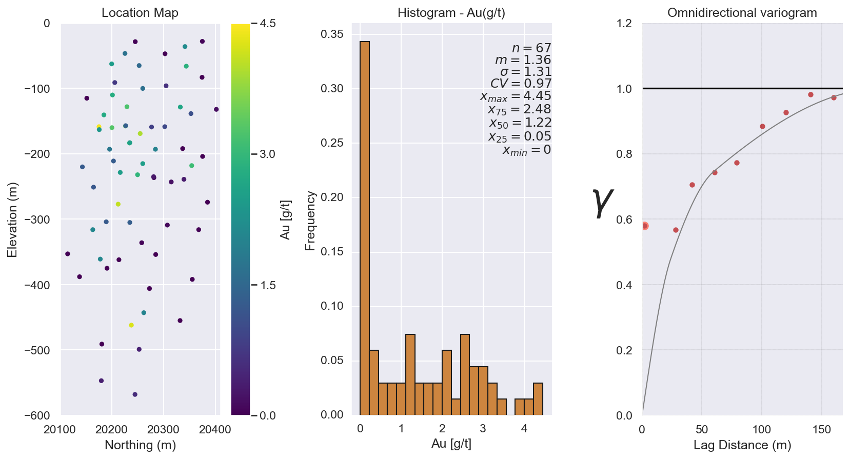
The first figure provides the location map of the intersections, the grade distribution, and the variogram model. The variogram was modeled with a low nugget effect, as the data pertains to the thickness of the vein structure, which is expected to vary smoothly.

Utilizing 25 data points in each local search, Figure 2 shows three subplots with the Ordinary Kriging estimates, KV, and KE. The KV plot indicates minimal variance at data points, which increases values when the data spacing increases. A lower KV indicates better estimation quality. In contrast, the Kriging Efficiency plot shows high efficiency at data points and lower values as the data spacing increases.

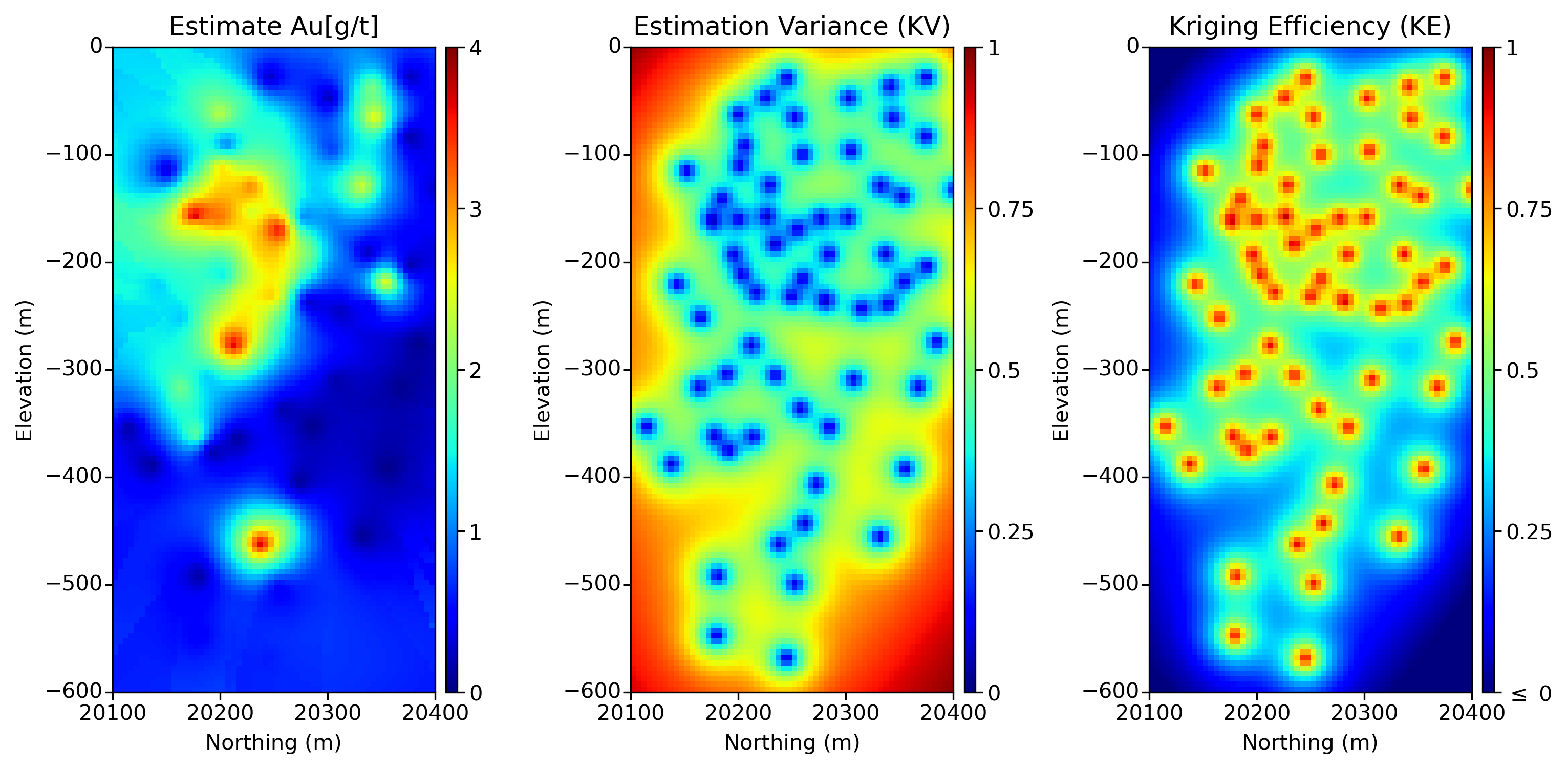
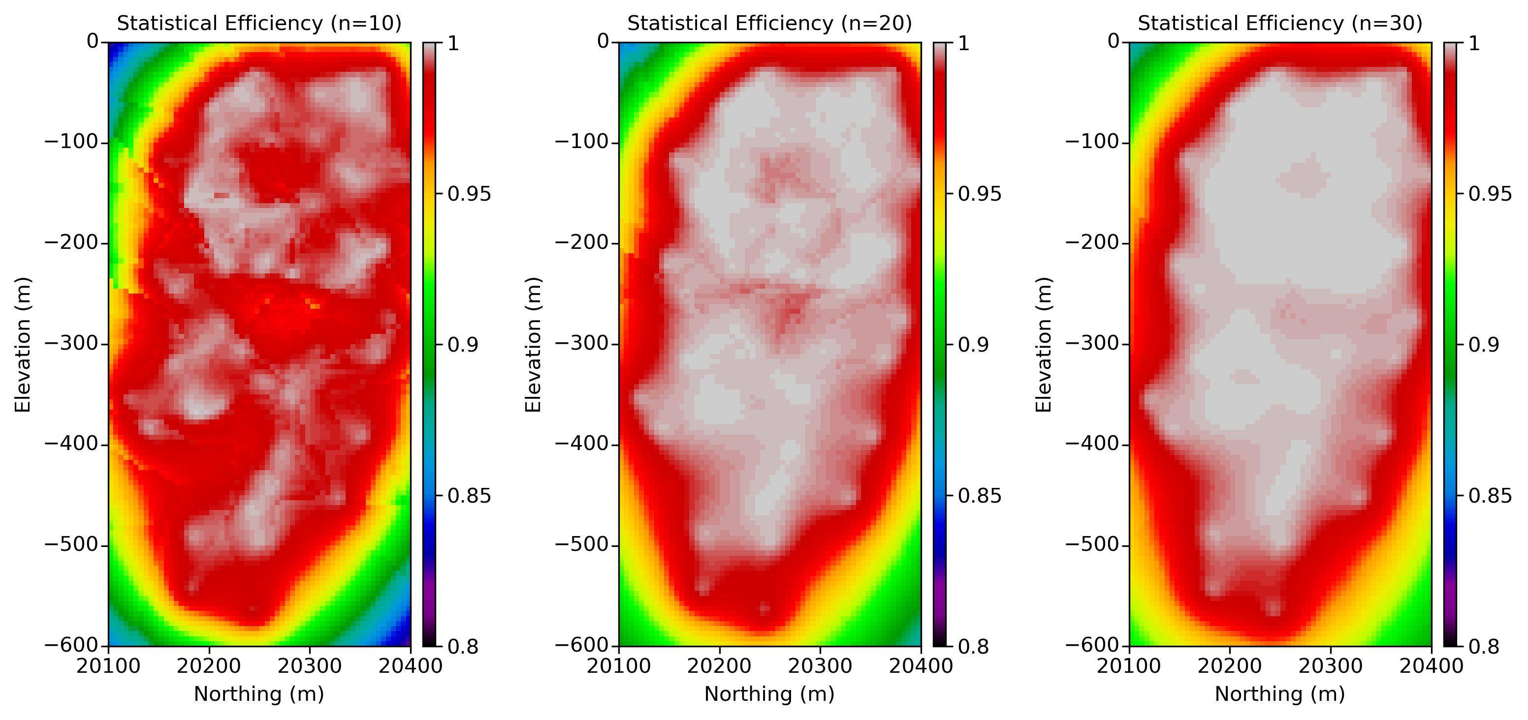
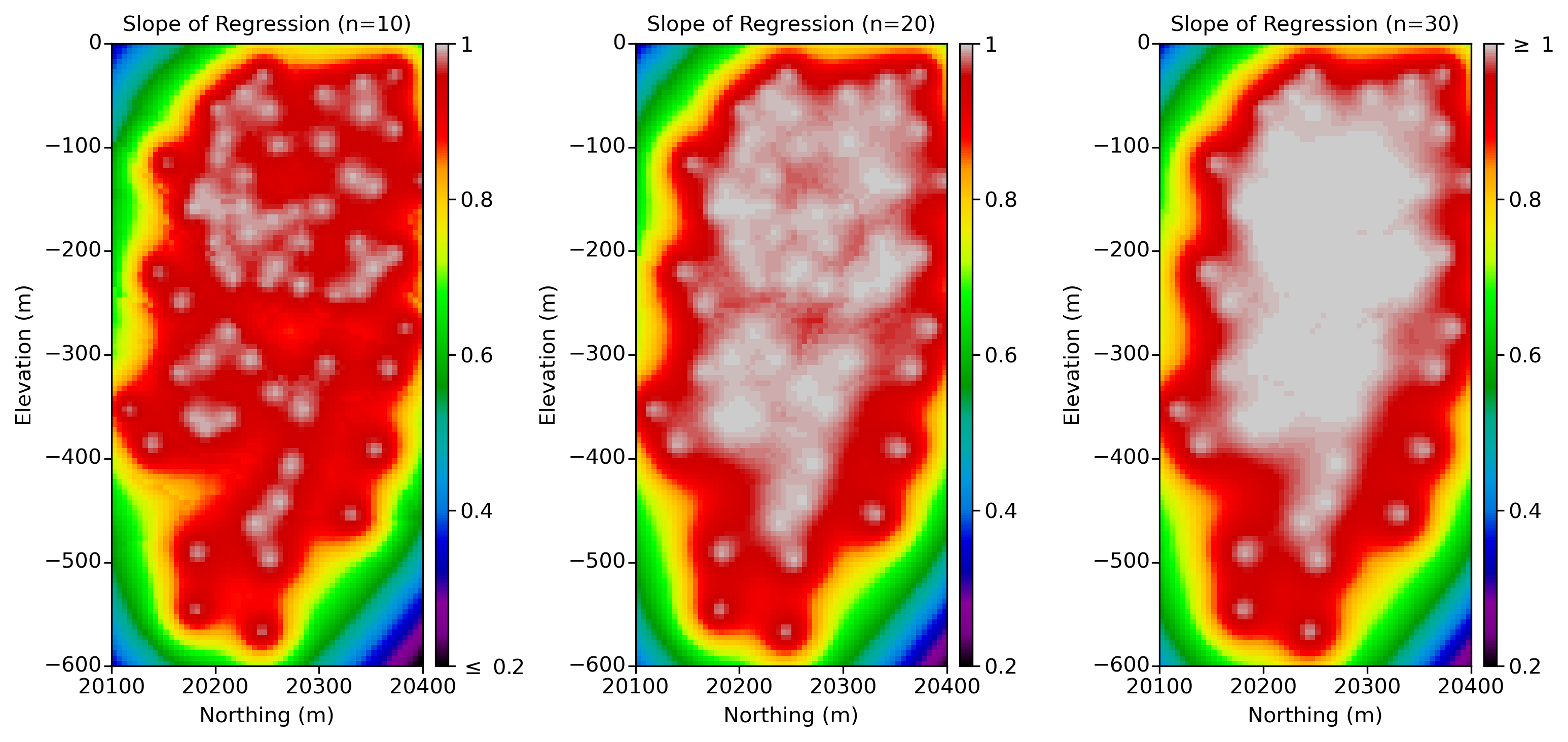
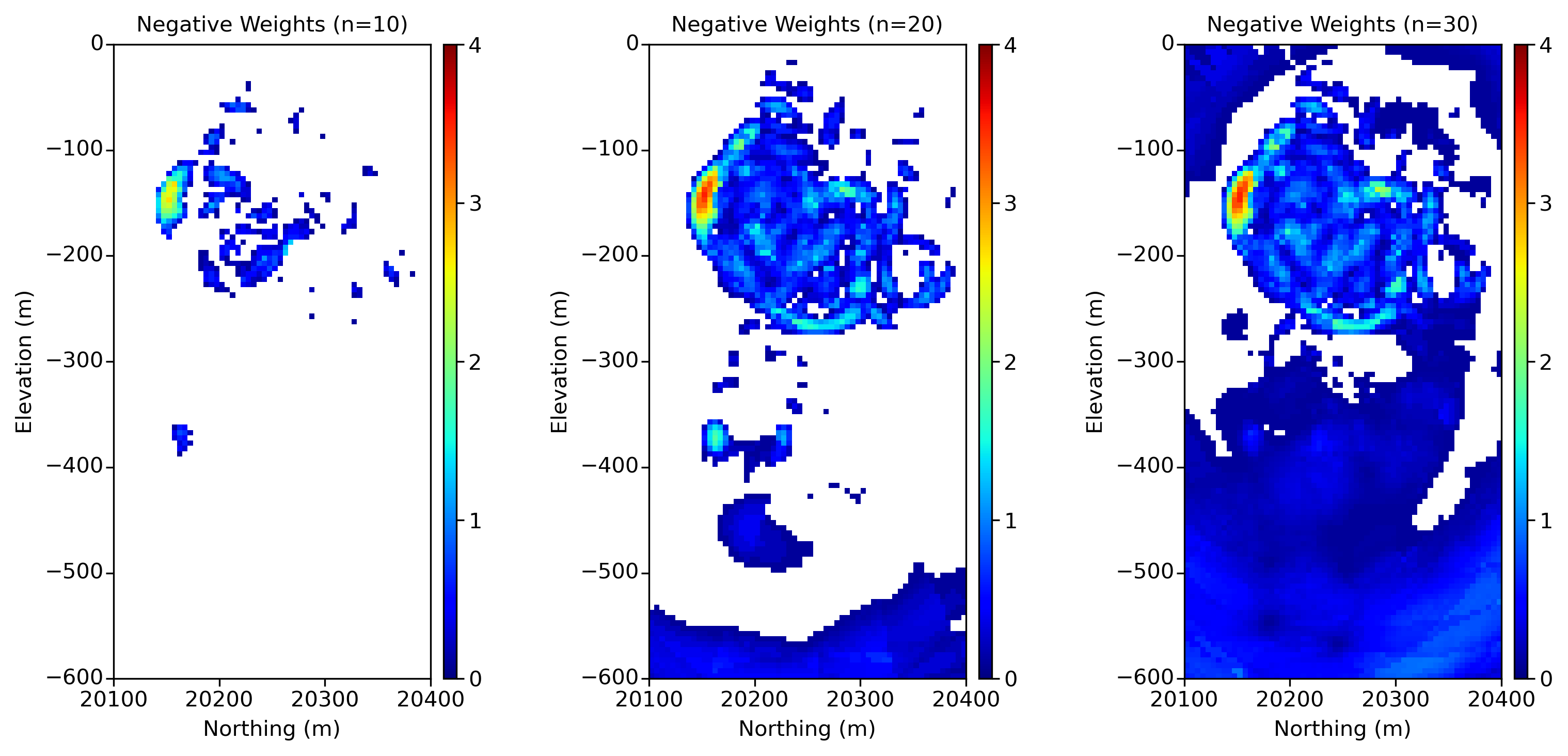
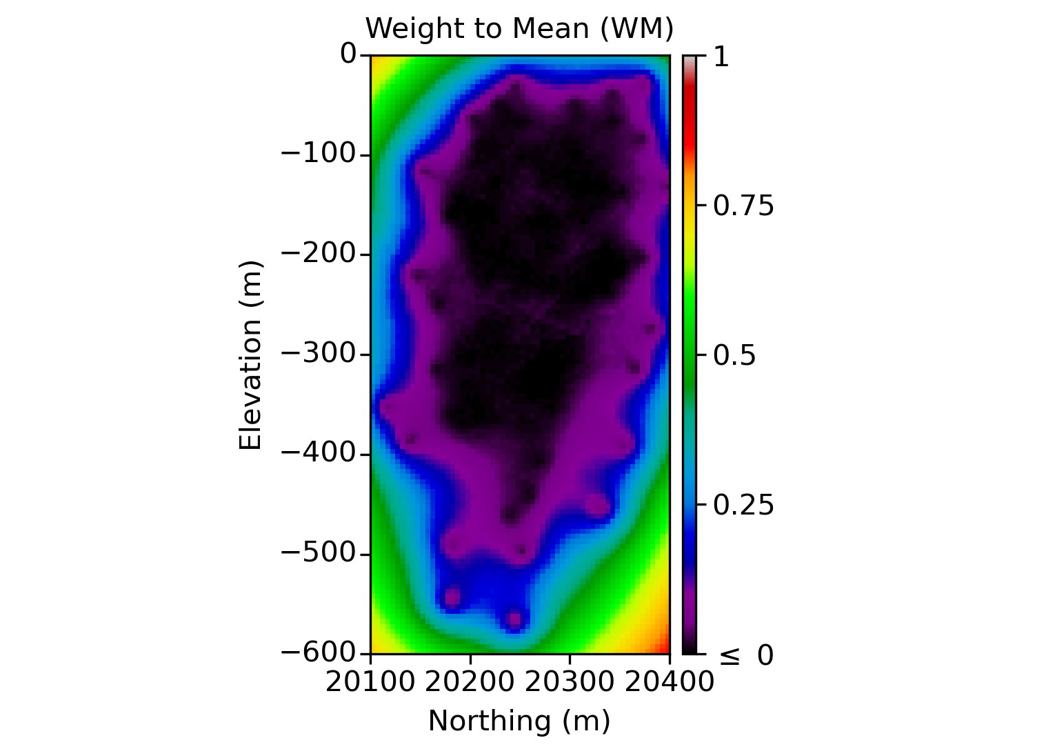
Figure 3 illustrates the improvement in SE with the inclusion of additional information (n=10, 20, 30) in the estimation process. The highest efficiency values are depicted in white. Using fewer data points results in greater variability compared to the true values, while efficiency improves with an increase in data, contributing to a more accurate estimation.

In Figure 4, the influence of data on the estimation quality relative to the true value is depicted. A SR less than 1 indicates an overestimation of high values and an underestimation of low values. Notably, with 30 data points, many values are very close to one.

Negative Weights are assigned to data screened behind closer data more highly correlated to the location being estimated and increase as more data is considered. Figure 5 illustrates the increase in negative weights as more data are considered. In regions with higher sample density, the Negatives weights per block increase with the addition of more data. Additionally, in areas of lower sample density or where there is no sampling, at least one negative weight is present. Blank space in the map represents blocks that there is only positive weights.

In Simple Kriging, the Slope of Regression (SR) is always one, but the Weight to the Mean (WM) is used as a diagnostic of data configuration and smoothing. Figure 6 shows this with larger WM values when data become more widely spaced. Slightly negative WM values may be encountered within regions of high data density, constituting less than 1% of the total.

Discussion

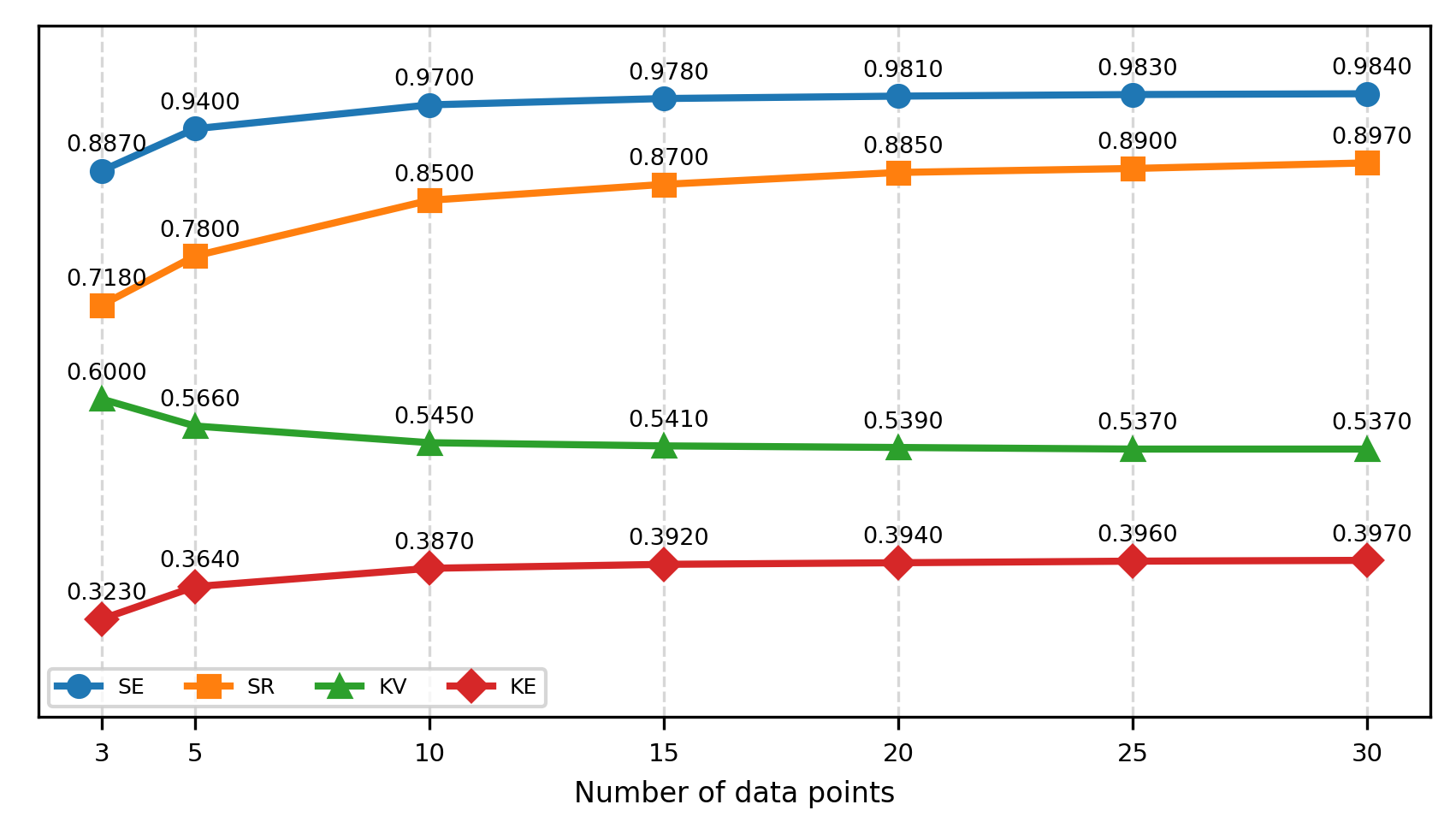
In Figure 7, the expected behaviour of KV, KE, SE, and SR are presented for Ordinary Kriging for a fixed block size of 5m x 5m as more data are included in the search. The QKNA measures systematically improve as more data is included. All measures show a monotonic behaviour, either increasing or reducing with the inclusion of more data, reaching asymptote values. This illustrates why QKNA does not provide definitive support on the selection of search parameters.

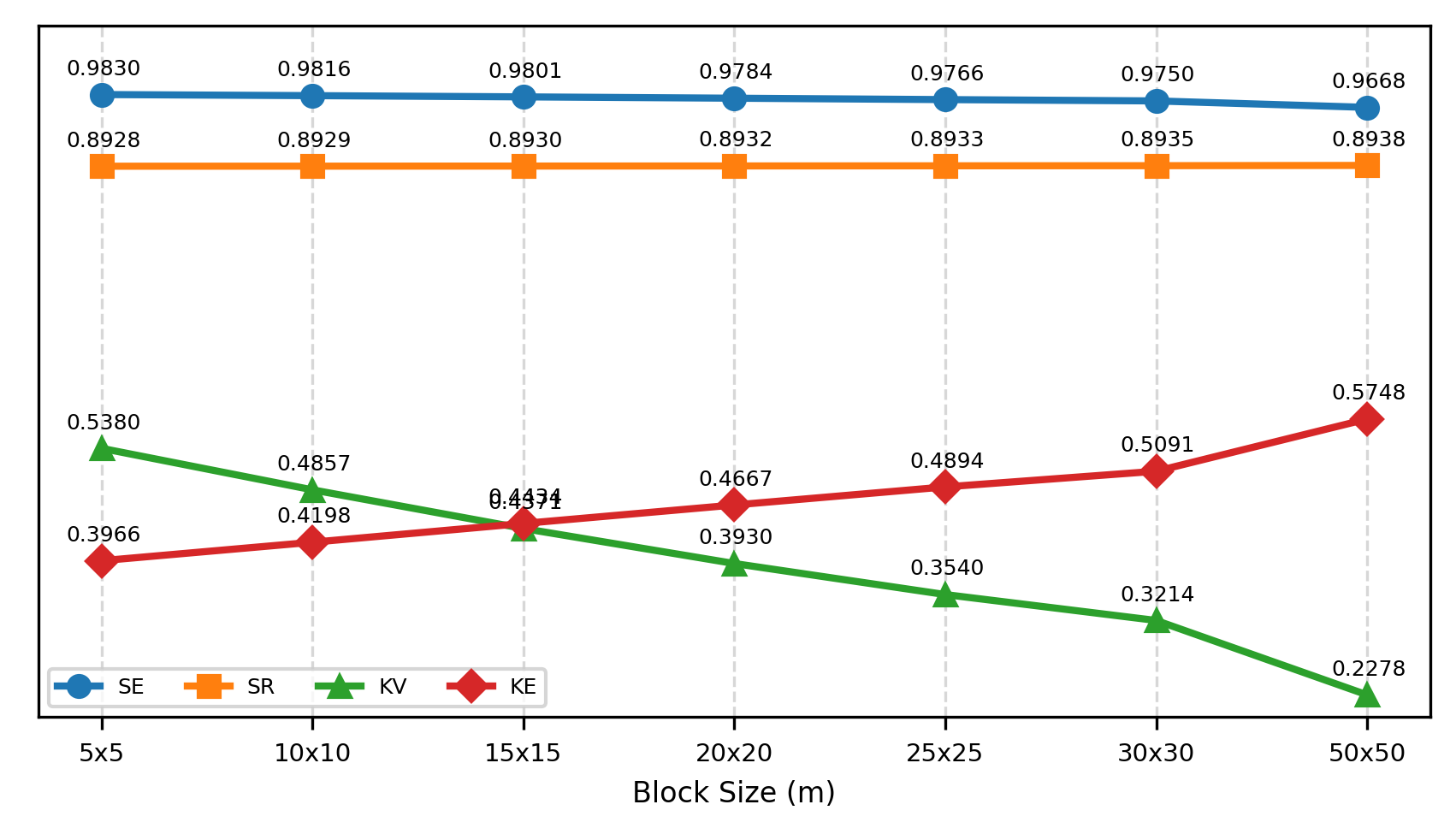
Regarding the block size, Figure 8 shows the QKNA measures for different block dimensions systematically improved. The number of data used for this figure remains the same. The SE and SR do not change to any significant degree, but the KV and KE systematically improve with larger block sizes. This illustrates why QKNA does not provide definitive support on the selection of block size.

From these measures of performance, Kriging estimation is always better with more data and with a larger block size. At a certain point, more data does not change the estimate; a maximum of 25 data for a 2D configuration and 50 for a 3D configuration seem reasonable. In the context of Kriging, there is an inherent level of smoothness that is acceptable according to the Kriging Plan (C. V. Deutsch & Deutsch, 2015). It is important to note that smoothness depends weakly on block size but depends strongly on the number of data used in ordinary kriging.

The selection for the search radius should be aligned with the medium to long-range variogram anisotropy. There are situations when a larger search radius than the range may be beneficial, allowing for the inclusion of data beyond the range to improve the estimation of the local mean in ordinary kriging. On the other hand, for zonal anisotropy, choosing a search radius less than the range is practical. In practical resource modeling, it is common to consider a multiple-pass search strategy with increasing search radius with increasing search pass. The QKNA measures of performance are sensitive to the details of the multiple pass search and, perhaps, could be used in the design of the multiple-pass search.

The determination of the block size in mining operations involves a careful evaluation of multiple factors, including engineering considerations, ore deposit geometry, equipment size, and data spacing. This decision holds substantial implications for pit design optimization and overall mine planning (Rossi & Deutsch, 2013). Aside from the considerations mentioned, the block dimensions chosen should deal with the smoothness implied in the upscaling process (Harding & Deutsch, 2019). Choosing a relatively small block size leads to slightly worse QKNA measures, but the estimates are more sensitive to the search setup than the block size.

In addition to the block size and search plan, the variogram has a large impact on the QKNA measures of performance. The variogram, derived from the available data, represents the underlying regionalized variable and cannot be easily altered to improve measures of performance. Geometric and zonal anisotropy will combine with the block size and orientation to change the measures. A variable with less structure will have a higher nugget effect, shorter range, or a variogram shape that increases quickly. In this case, there will be fewer negative weights, but all other measures of performance will appear worse.

Conclusions

Achieving a low Kriging Variance (KV), high Kriging Efficiency (KE), high Statistical Efficiency (SE), Slope of Regression (SR) close to one, few Negative Weights (NW), and a low Weight to the Mean (WM) indicates a robust kriged estimates. The utilization of these Quantitative Kriging Neighborhood Analysis (QKNA) measures serves as a tool in understanding the performance of a block model. QKNA measures implicitly suggest using many data in the estimation of large blocks, but there are many practical considerations to be considered. A major decision in the choice of a kriging plan is the purpose of the estimate. Final estimates in grade control should place emphasis on these measures. Long range resource estimates would have to consider the information effect and the risk of excessive smoothing if these measures are given priority.

References