Learning Objectives

• Classify estimates according to their purpose: interim estimation, final decisions, visualization, and probabilistic prediction.
• Know best practice in choosing a fit-for-purpose kriging plan.
• Understand stationarity, kriging performance measures, and other concerns when choosing a kriging search plan.
• Understand the techniques and comparisons (source code available).

Introduction

This lesson relates primarily to mining where estimation is still widely practiced for resource and reserve estimation. Kriging is the primary technique for the estimation of grades. Kriging is a linear unbiased estimator that minimizes the estimation variance using a site-specific variogram model of spatial variability accounting for anisotropy and other spatial features (Journel & Huijbregts, 1978). The number of data and locations of data used to inform the estimate compose the kriging search plan. The kriging search plan is typically restricted due to concerns about computational time, stationarity, conditional bias, and histogram reproduction. These restrictions and concerns are the subject of this lesson.

There is no doubt that the prerequisites to kriging are more important than the details of the kriging plan. These prerequisites include ensuring data quality, compositing, managing outliers, subdividing the data into reasonable subsets (domains), establishing an appropriate coordinate system for estimation, choosing the correct block size for estimation, and managing large scale trends and contacts between estimation domains. Nevertheless, details of the kriging plan are important provided these prerequisites have been met in a reasonable fashion.

The choice of a kriging search plan is dictated by the purpose of the estimate; there is no universal best kriging plan. Best practice in choosing a kriging search plan depends on the estimate purpose. This lesson addresses the selection of a kriging search plan for four types of estimates, and discusses concerns of stationarity, kriging measures, and other common practices.

Purpose of the Estimate

We classify the purpose of estimates into four categories: 1) interim estimates, 2) final estimates, 3) visualization and trend models, and 4) probabilistic predictions. Each of these estimation purposes has a different set of criteria for choosing the best kriging search plan.

Interim Estimates

Interim estimates are estimates awaiting more data. Early in the life cycle of a mineral deposit there are relatively few data available for estimation. At the time of mining, many more data are available in the form of blast holes and drill holes. This disparity in available data is termed the information effect (Rossi & Deutsch, 2013). One goal of interim estimates is to provide close estimates of ore tonnage, ore grade and waste tonnage within reasonably large production volumes (sometimes called mining panels). A too-large search will result in over smoothing of the grades and inaccurate estimation of tonnage and grade. The search could be restricted to improve the estimate of tonnage and grade; however, this will come at a cost of conditional bias. This cost is not severe since interim estimates are not final estimates; these may be used in the mine plan and for technical and economic evaluation; however, additional information will be available prior to mining and final grade control decisions.

Final Estimates

Final estimates are an interesting time in a mining context; the classification of material as ore or waste (grade control) will have a direct and final economic impact on the mine. The emphasis is on the minimization of conditional bias, minimization of mean squared error and minimization of Type I and Type II errors (Isaaks, 2005). Final estimates are constructed with the goal of making the best possible estimate according to our mean squared error criterion. Final estimates are made with all data that will be available; no additional data is expected prior to use of the estimate.

Interim estimates in an underground mining context may be considered as near-final estimates depending on the flexibility of the mining method. If there is little future flexibility, then concerns of conditional bias and Type I/II errors are important and estimates could be considered as final.

Visualization and Trend Model Estimates

Visualization and trend models include all models where the goal is a smooth, interpretable map of the properties of interest. The purpose is to understand the entire spatial distribution of the property being estimated, not discrete estimates one at a time as in resource and reserve estimation. Visualization estimates are commonly used with geologic mapping to evaluate our conceptual geologic model, and draw conclusions on the presence and nature of trends in the data. The requirement for these models is that they be free of numerical artifacts to permit reliable interpretation.

Probabilistic Prediction Estimates

Probabilistic predictions, including multigaussian kriging (Verly, 1984) and indicator kriging (Journel, 1983) within an estimation or simulation context constitute the fourth type of estimate. In this case, the kriging equations are used to construct a conditional probability distribution at an unsampled location in the presence of correlated data. For multigaussian kriging, the kriging equations are typically referred to as the normal equations. The normal equation formalism is used throughout Gaussian and probabilistic geostatistics. The goal of probabilistic predictions is to infer the most accurate set of probabilities, free from any conditional bias or artifacts. Smoothing is not a concern since the predicted distribution represents the uncertainty and variability.

Best Practice

As discussed earlier, best practice for all estimate types is to only apply estimation within a decided stationary domain. All prerequisites including composite length selection, block size selection, and stationary domain selection must be considered prior to estimation. The decision of stationarity has typically been made long before the application of kriging; this decision is made as soon as data are grouped together for analysis.

Best Practice: Interim Estimates

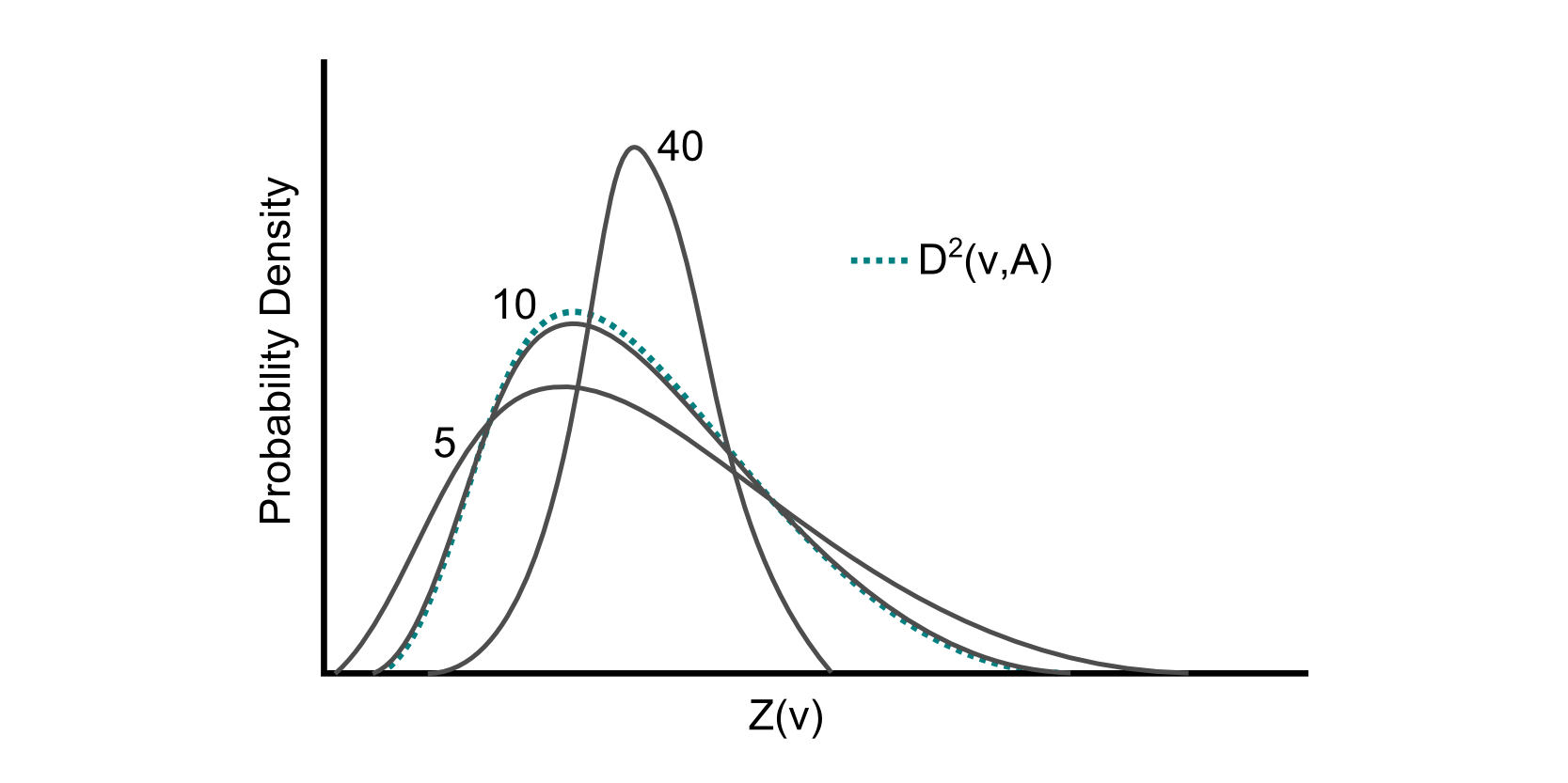
Best practice for interim estimates is to use a restricted search with ordinary kriging to compute estimates that closely matches the anticipated grade tonnage curve (Parker, 1979). Ordinary kriging provides direct control on the smoothing; a small number of data in the search will lead to a histogram of estimates with little smoothing. The spatial distribution of estimates will always be smooth, but the histogram of estimates can be controlled. The search should be restricted by limiting the maximum number of data used to compute the kriging estimate. A known histogram of values at the scale of interest (such as the selective mining unit size) is targeted. This histogram may be calibrated from production data, if any are available, and by volume variance relations. The impact of restricting the number of search data is sketched in the following figure.

There are additional considerations when restricting the search for ordinary kriging. The number of data used from each drill hole may be restricted. This is common when making estimates in a 3D domain with vertical drilling and a relatively short composite length; much more data is collected in the vertical direction compared to the horizontal plane. A maximum per drill hole avoids using data from only a single drill hole when making an estimate with very few data. The search range may also be restricted; the range of the variogram is a common choice for the search range, but in practice restricting the number of data used in an estimate is a more reliable method of restricting the search.

The consequence of restricting the number of data used in the kriging estimate is conditional bias. High grade areas are overestimated because local high grade values are given more weight. Low grade areas are correspondingly underestimated because of additional weight given to low grade values. There will be no global bias and there should be no bias in ore tonnes and ore grade at the targeted cutoff. Conditional bias is not a problem for interim estimates as they will be updated before final decisions are made; however, care should be taken not to use this type of estimate for final decisions.

Best Practice: Final Estimates

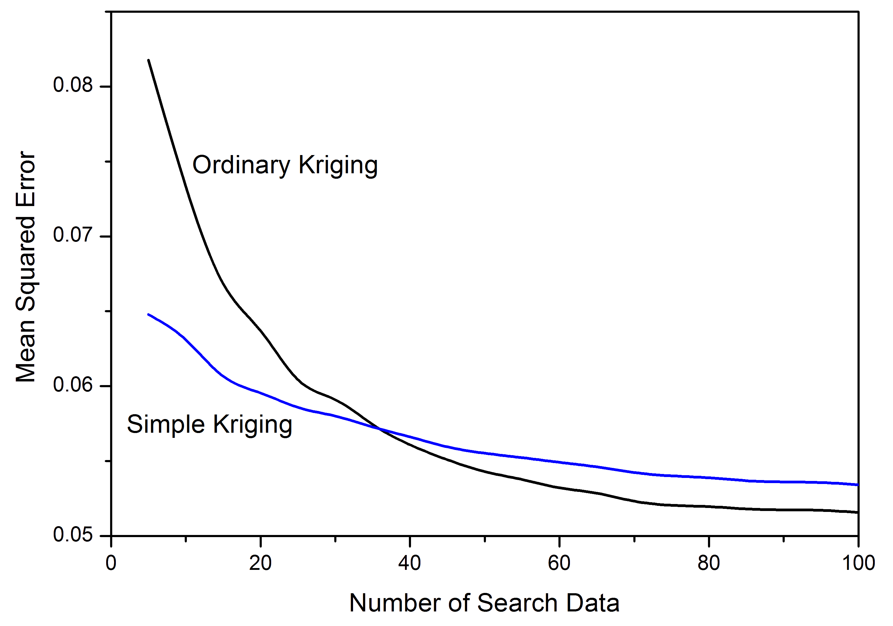
The kriging plan for final estimates is chosen to minimize mean squared error and conditional bias. Best practice for making a final estimate is to use ordinary kriging with a large number of search data to minimize the estimation error. Simple kriging is typically not as effective due to an overly strong dependence on the global mean. This is shown in the following figure plotting the mean squared error from cross validation as a function of the maximum number of search data used in kriging a copper porphyry deposit. Using additional search data results in only a marginal improvement past a certain amount of data, but does not result in a worse estimate. Specific concerns about stationarity and performance measures are addressed later in this lesson.

The specific number of search data chosen when making a final estimate is a function of the computational time required for the estimate. Choosing 40 search data in a 3D estimation context, or 24 in a 2D context, is often a reasonable number to balance the computational time and desire for the best estimate. The number of data used weakly depends on the support of the data. More data of small support could be considered.

The search range should be set at the variogram range or even larger to include the required number of data. Often, production data are reasonably closely spaced and the effective search range that will get the required number of data is reasonably small. Limiting the kriging search range to an arbitrary value that excludes data from the estimate is not best practice. The search radius should consider the variogram anisotropy.

Best Practice: Visualization and Trend Model Estimates

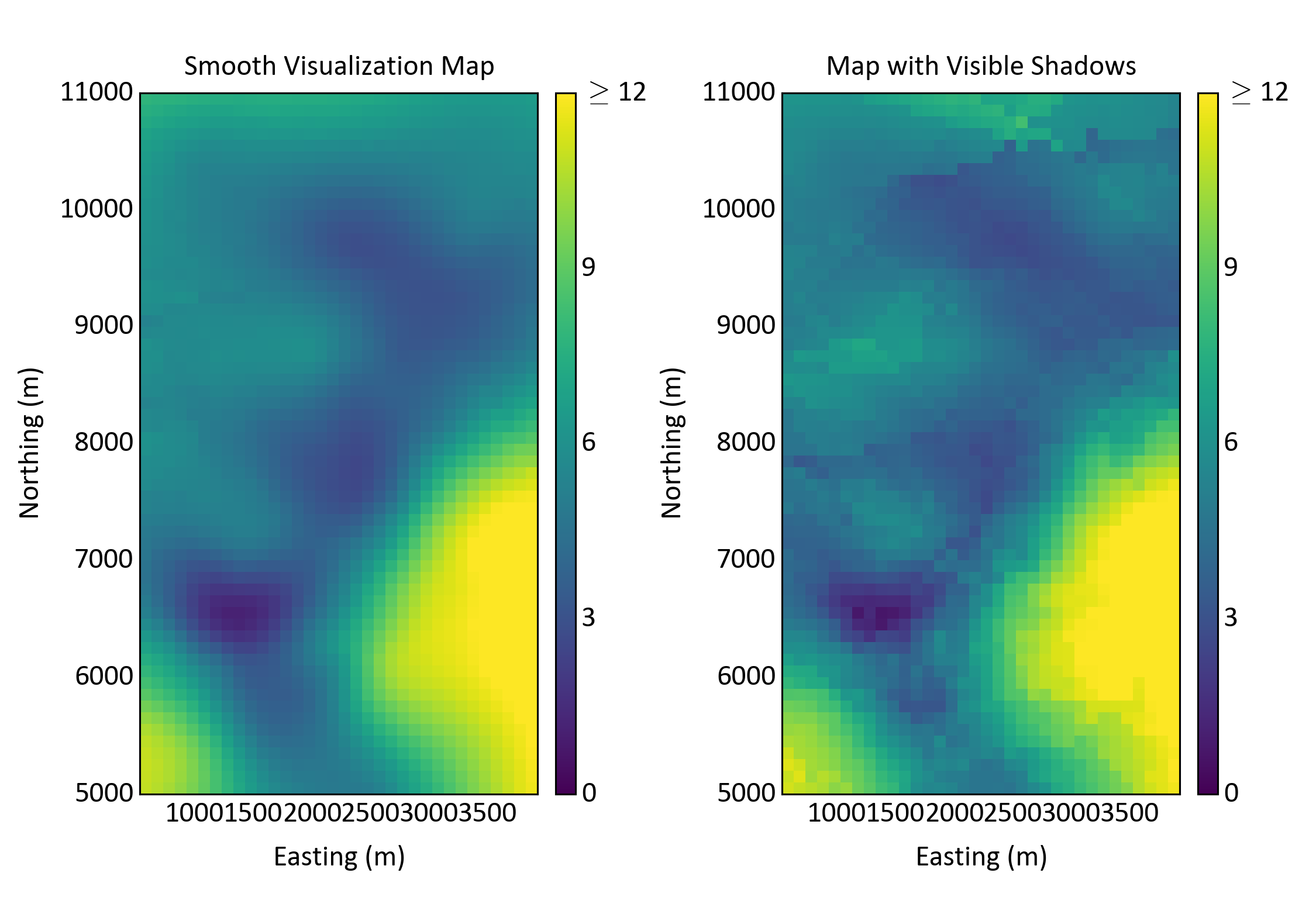
Best practice for visualization and trend model estimates is similar to final estimates. The goal of a smoothly varying interpretable map is best met by kriging with a large search. Typically simple kriging is used to reduce the impact of local means in sparsely sampled and peripheral areas which could influence our interpretation. Ideally global kriging is used, but a very large number of search data may be used if there are too many data for global kriging (about 10,000). Limiting the number of search data results in “shadows” and numerical artifacts, as shown in the following figure. Artifacts are visible particularly in the upper portion of the map which is undesirable for interpretation.

Best Practice: Probabilistic Prediction Estimates

Probabilistic prediction estimates, including multigaussian and indicator kriging, are made with the goal of inferring the best probability distribution. Best practice is to use a large search to include all data that should influence the predicted probability distribution. Simple kriging is the correct kriging type for prediction in a multivariate Gaussian context. This is true for both multigaussian kriging for local uncertainty characterization or within simulation. Ordinary kriging is more often applied for indicator kriging. Simple kriging is required to ensure covariance reproduction; however, stationarity concerns are often considered more important and there are no strong theoretical requirements as with the multivariate Gaussian distribution. Concerns such as over-smoothing for interim estimates are not applicable in a probabilistic estimation context where the parameters of probability distributions are being estimated. Limiting the number of search data results in suboptimal estimates of the probability distributions.

Considerations

As kriging has been widely applied since the 1960s, a large number of specific considerations have been discussed by geostatistical practitioners. Some of these considerations, including stationarity, kriging performance measures, and multipass kriging are discussed here as they relate to best practices for estimation.

What About Stationarity?

One might think that the number of search data should be reduced to account for local fluctuations in stationarity. The logic is that a limited search will produce a better estimate of the local mean for estimation. This has not been observed in practice; using more search data does not result in a worse (higher mean squared error) estimate. The apparent improvement due to locally adapting to variations in the mean is not backed up in jackknife, cross validation, or when checking with production data. Final estimates benefit from a reasonably large number of data despite concerns about smoothing.

What About Kriging Performance Measures?

Measures of kriging performance are variably popular. The slope of regression, kriging efficiencies, the prevalence of negative weights, and weight to the simple kriging mean are often cited as important measures and used in the selection of kriging plans (Vann, Jackson, & Bertoli, 2003).

The slope of regression of estimates against true values is used as an approximation of the conditional bias of the kriging estimate. Simple kriging, which is an unbiased estimator, has a slope of regression of exactly one. In ordinary kriging, where a Lagrange multiplier is used, the slope of regression is typically less than one indicating a conditional bias. Increasing deviation from a slope of one indicates an increased conditional bias. Although the slope of regression is often documented; it is of little utility when choosing a kriging search plan. In an interim estimation context, the most important parameter is matching the desired histogram. In a final, visualization, or probabilistic estimation context, a very large number of search data is used to minimize the mean squared error and conditional bias is essentially zero. Ideally the conditional bias is eliminated for a final estimate, but this may not always be possible (Isaaks, 2005).

Kriging efficiency (Krige, 1997) is a measure of the proportion of variance explained. The related measure of the statistical efficiency of kriging (Deutsch et al., 2014) provides a measure of the effectiveness of an estimator relative to the optimal global simple kriging estimator. These measures may be mapped over the domain of interest. Application of these efficiency measures for decision making is challenging due to large differences between mineral deposits (Rossi & Deutsch, 2013). When mapped, the kriging efficiency is relatively low in sparsely sampled areas, and high in densely sampled areas. It is evident that estimates are worse when data are widely spaced. The kriging variance is a robust measure of data spacing and may be used in place of the kriging efficiency.

What About Negative Kriging Weights?

Negative kriging weights are applied to data that are screened behind other data more highly correlated to the location being estimated. Most negative kriging weights improve estimation because local trends in the data are more accurately interpolated. There are concerns, however, when the negative weights become extreme and when they cause negative grade estimates. Clearly, negative grade estimates should be reset to zero. A significant proportion of negative estimates in an estimated model implies that the variogram may have been modeled too continuously.

Closely related to negative kriging weights is the so-called string effect where samples at the ends of a string of data receive more weight than data within the string. These strings of data are caused by the search for data along a drill hole. Cross validation should identify this problem with some large errors. Limiting the number of data used in the kriging plan per drill hole will mitigate this problem.

What About…?

There are some other considerations. In general, except for interim estimates, the practitioner should err on the side of using more data in the kriging. The kriging equations will sort out the optimal weight for the data; data far from the unsampled location or screened by closer data will not receive any significant weight.

The use of multiple search passes is aimed at the important problem of classification and at restricting estimation to use nearby data in areas of more data. This practice introduces artifacts where one search strategy ceases to be satisfied and another is considered. Choosing a fairly large search and restricting the maximum number of data accounts for varying data density. The estimates may be better classified by data spacing calibrated to simulation-based uncertainty measures.

There may be a need to carefully clip a kriged model to avoid estimating too far from the data, below the deepest drill holes or at the margins. There may be a need to account for soft boundaries and many other practical details. These concerns warrant additional discussion, and will be addressed in future lessons; this lesson forms an introduction to choosing a kriging plan.

References