Cite this lesson as: Carvalho, D., & Deutsch, C. V. (2017). An Overview of Multiple Indicator Kriging. In J. L. Deutsch (Ed.), Geostatistics Lessons. Retrieved from http://geostatisticslessons.com/lessons/mikoverview
An Overview of Multiple Indicator Kriging
Dhaniel Carvalho
University of Alberta
Clayton Deutsch
University of Alberta
January 27, 2017
Learning Objectives
- Understand the principles and place of Multiple Indicator Kriging (MIK).
- Comprehend the steps and decisions to implement MIK.
- Appreciate limitations and post processing of MIK-derived distributions.
Introduction
The key objectives of multiple indicator kriging are to (1) manage highly variable natural phenomena without cutting high values or nonlinear transformation, and (2) estimate the local distribution at each unsampled location to provide risk-qualified estimates (Journel, 1983). The aim is to model complex mineralization with non-Gaussian structure, including asymmetric spatial continuity of high and low values.
The original data \(Z(\textbf{u})\) are considered in binary transformations within a chosen stationary domain \(A\), based on defined \(Z_k\) thresholds. Often between \(K = 7\) and \(K = 15\) thresholds are selected. This discretizes the range of variability of the continuous variable \(Z\). Consider the random variable \(Z(\textbf{u})\) at a location (\(\textbf{u}\)) within a stationary domain \(A\):
\[ F(\textbf{u}; z_k) = I(\textbf{u}; z_k) = \begin{cases} 1, & \mbox{if $Z(\textbf{u}) \le z_k$} \\ 0, & \mbox{otherwise} \end{cases}, \quad k=1,\ldots,K, \quad \textbf{u} \in A\]
The prior global distribution at K thresholds can be estimated by a weighted average of indicator data:
\[F^*(z_k) = \displaystyle\sum_{\alpha=1}^n w_\alpha i(\textbf{u}_\alpha; z_k) , \quad k=1,\ldots,K \]
where \(w_\alpha\) are declustering weights applied to the \(n\) indicator data at each threshold \(i(\textbf{u}_\alpha;z_k)\). There is no resolution preserved between thresholds as the only points of the probability distribution used are at the indicator thresholds.
Some important prerequisites to consider before applying MIK are: (1) the domain should be as stationary as possible with manageable transitions to other domains, (2) outlier values must be managed as usual although MIK is more resistant to outliers than most methods, (3) the data should be composited to a reasonable length to remove excessive high frequency variations while preserving important short scale variability, and (4) appropriate declustering weights should be computed for a representative global distribution.
Global Histogram and Thresholds
Choosing thresholds is the first step of multiple indicator kriging. The number of thresholds is normally chosen between 7 to 15; considering too many may induce more order relation problems and too few thresholds would result in low resolution of the predicted distributions. Some criteria for choosing the thresholds include:
Commonly start with nine thresholds defining deciles of the global distribution
Move the thresholds to correspond to interesting inflection points on the cumulative distribution function
Remove some low thresholds depending on the cutoff grade and add some high thresholds to define approximately equal quantity of metal in the upper classes
Move the thresholds so one matches the specified cutoff grade
Intervals should have enough data for a robust estimation; perhaps a minimum of 4 to 5% of the data.
The variogram for the indicator data should change in a reasonable way from one threshold to the next. Additional thresholds may be needed if the indicator variogram changes abruptly. Some thresholds could be dropped if the variograms do not change and the resolution is not required.
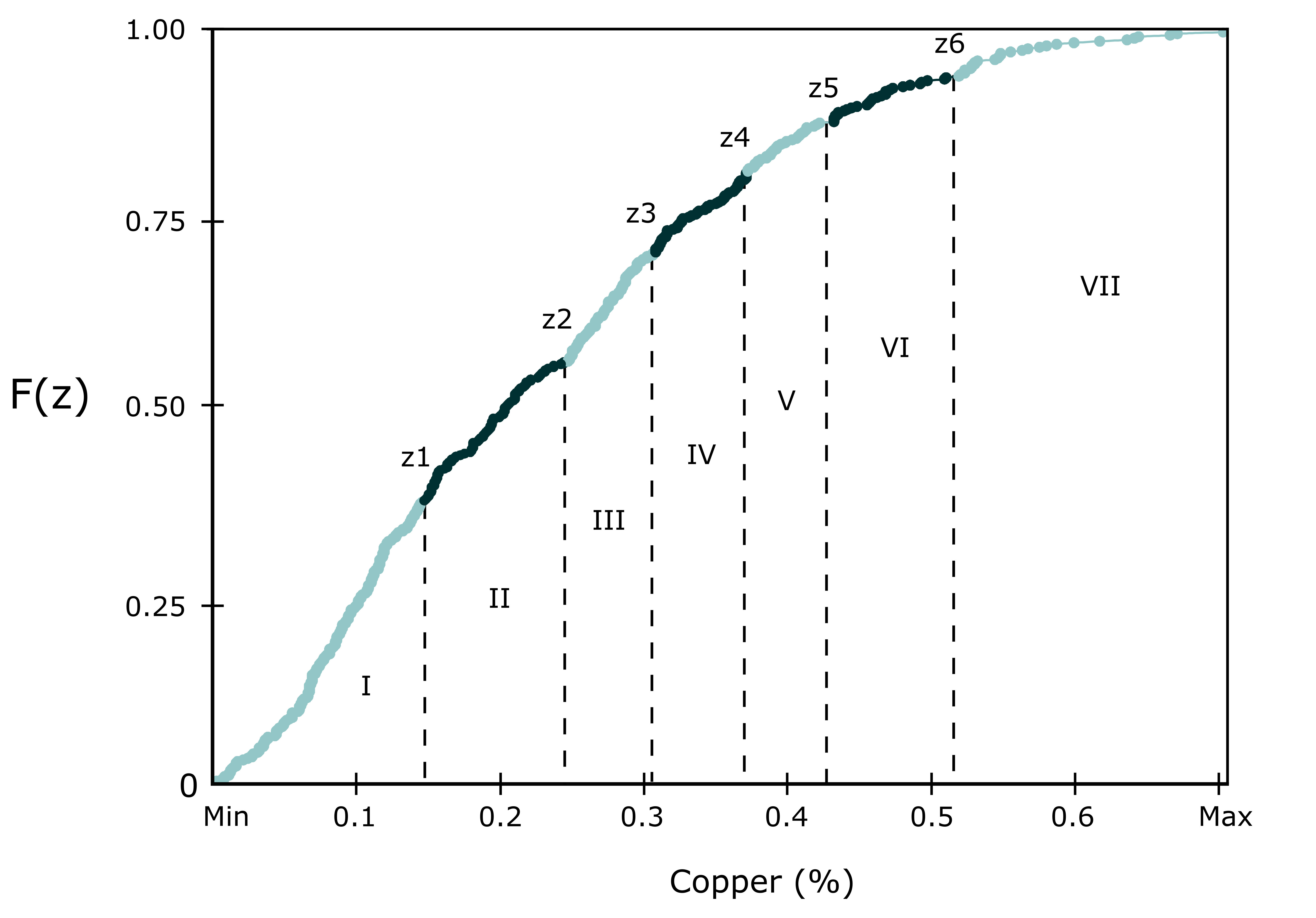
The figure shows a declustered global CDF from a copper deposit. The table below summarizes the thresholds and resulting classes. Note that inflections are mostly reproduced, there is similar metal content in the classes, the economic cutoff grade is the second cutoff and there are a reasonable number of data in each class.
| Classes | Grade From | Grade To | CDF | Probability | No. Samples | Metal Quantity |
|---|---|---|---|---|---|---|
| I | 0.01 | 0.15 | 0.37 | 37.0% | 184 | 12.7% |
| II | 0.15 | 0.25 | 0.56 | 18.7% | 93 | 14.3% |
| III | 0.25 | 0.31 | 0.70 | 14.3% | 71 | 15.8% |
| IV | 0.31 | 0.38 | 0.80 | 10.5% | 52 | 14.2% |
| V | 0.38 | 0.44 | 0.88 | 7.8% | 39 | 12.6% |
| VI | 0.44 | 0.53 | 0.95 | 7.0% | 35 | 13.6% |
| VII | 0.53 | 7.74 | 1.00 | 4.6% | 23 | 16.7% |
Indicator Variograms
It is necessary to model directional variograms for the indicator data at each threshold. These variograms are often well behaved as the data are only 0s and 1s. Nevertheless, carefully choosing orientations and variogram parameters is still necessary to acquire stable variograms. The indicator variograms should be standardized to make it easier to analyze, compare and model the indicator variograms.
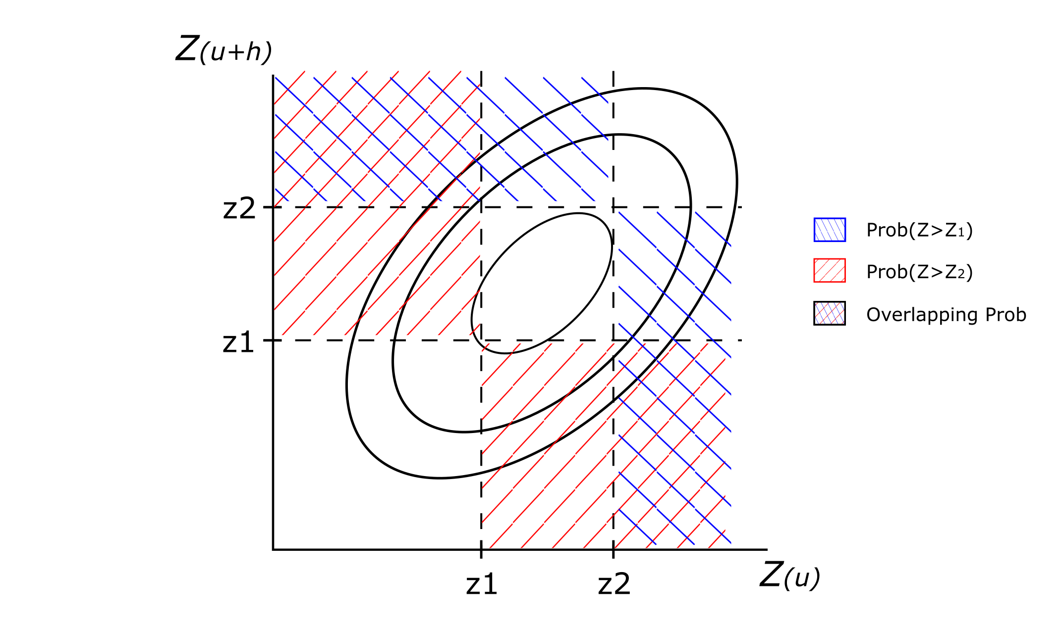
Any licit variogram structure that rises linearly at the origin such as exponential and spherical can be used for modeling the variograms. It is convenient to use the same type for all indicator variograms to ensure consistent changes. The indicator variograms, after all, relate to the same underlying continuous variable. Transitions between the indicator variograms are expected to be smooth in terms of variance, anisotropy, and ranges. To check these transitions from one indicator to the next, the ranges, nugget effects and anisotropy can be plotted versus the threshold number. There should be no abrupt discontinuity between variograms of consecutive thresholds. The figure below is an h-scatterplot indicating the contribution to two indicator variograms at thresholds z1 and z2. Note that they share much of the same structure. Changing from z1 to z2 amounts to a loss of some points and a gain of some others; therefore, the indicator variogram for nearby thresholds cannot be too different.
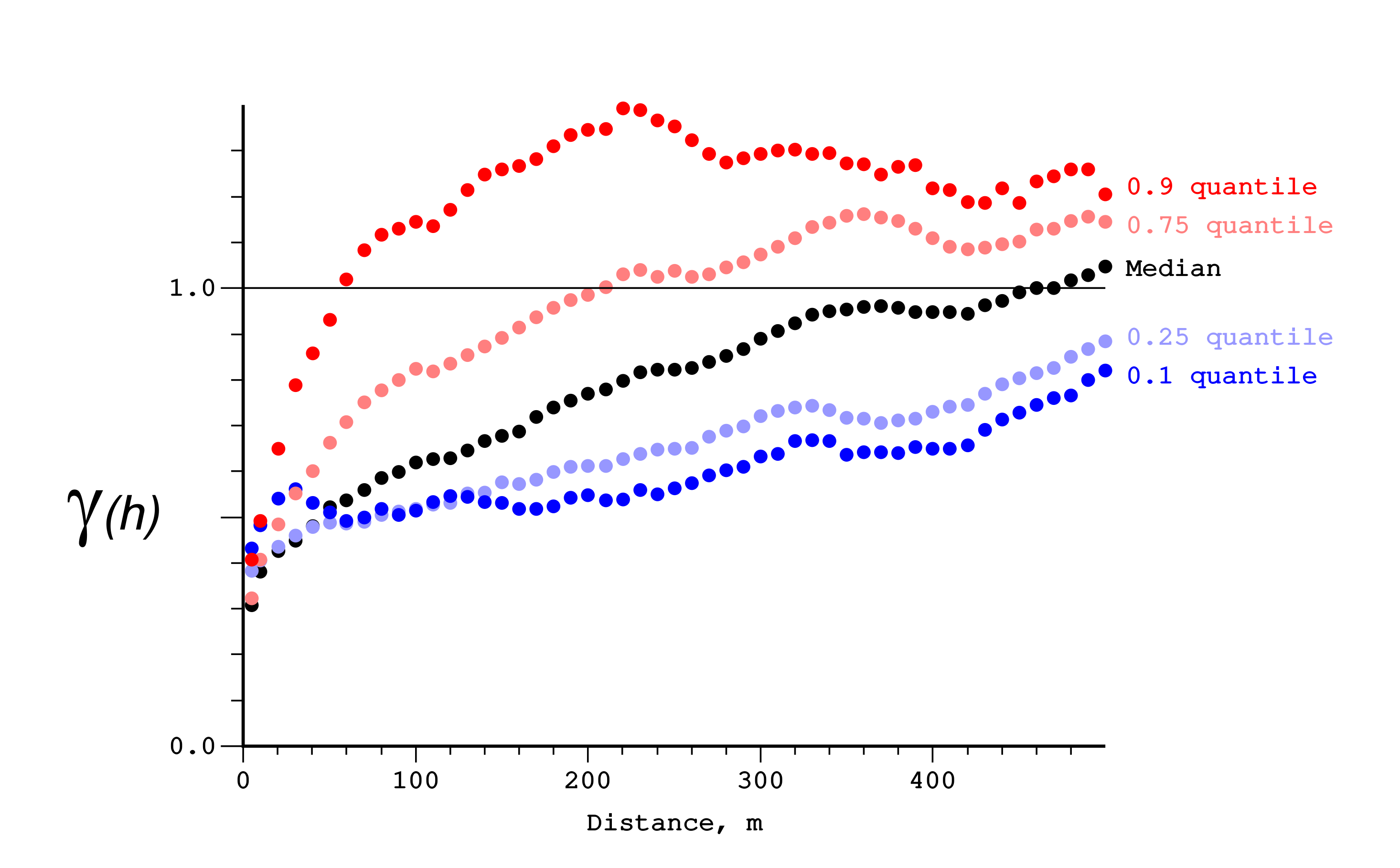
It is also important to note that there might be strong destructuration on higher thresholds variograms and weaker on lower ones. The figure below shows some disturbances on nugget effect from lower quantiles and intense range decrease for higher quantiles.
Indicator Kriging
There are some recommendations in the Lesson on Introduction to Choosing a Kriging Plan. It is advisable to use the same search plan with a reasonably large search neighborhood and number of samples. Changing the search parameters for the thresholds could create artifacts and unstable estimates of the probabilities. The local distribution for each \(\textbf{u}\) location is estimated at the \(K\) thresholds. Ordinary kriging is almost always used:
\[ F^*(\textbf{u}; z_k) = i^*(\textbf{u};z_k) = \displaystyle\sum_{\alpha=1}^n\lambda(\textbf{u};z_k)i(\textbf{u}_\alpha;z_k), \quad k=1,\ldots,K, \quad \textbf{u} \in A \]
The ordinary kriging weights \(\lambda\) change with the indicator variograms for each threshold.
Order Relation Correction
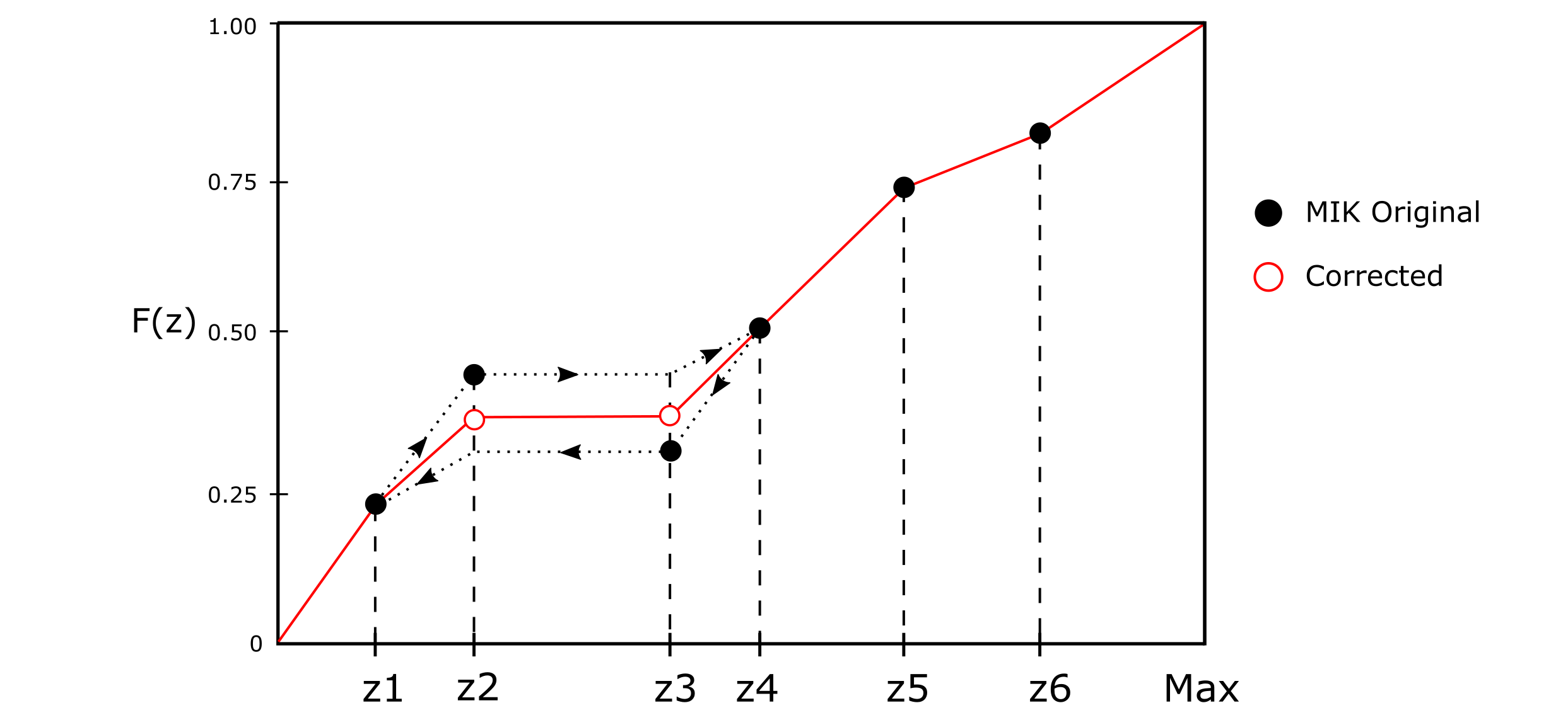
As the thresholds are estimated separately, the estimated conditional CDF values may not satisfy the order relations for a valid CDF (Journel, 1983). The source of these problems is related to poorly modeled variograms, inconsistent kriging plans, negative kriging weights and a lack of data for some thresholds. One reasonable method for correction is to use the algorithm for averaging the upward and downward corrections (Deutsch & Journel, 1998).
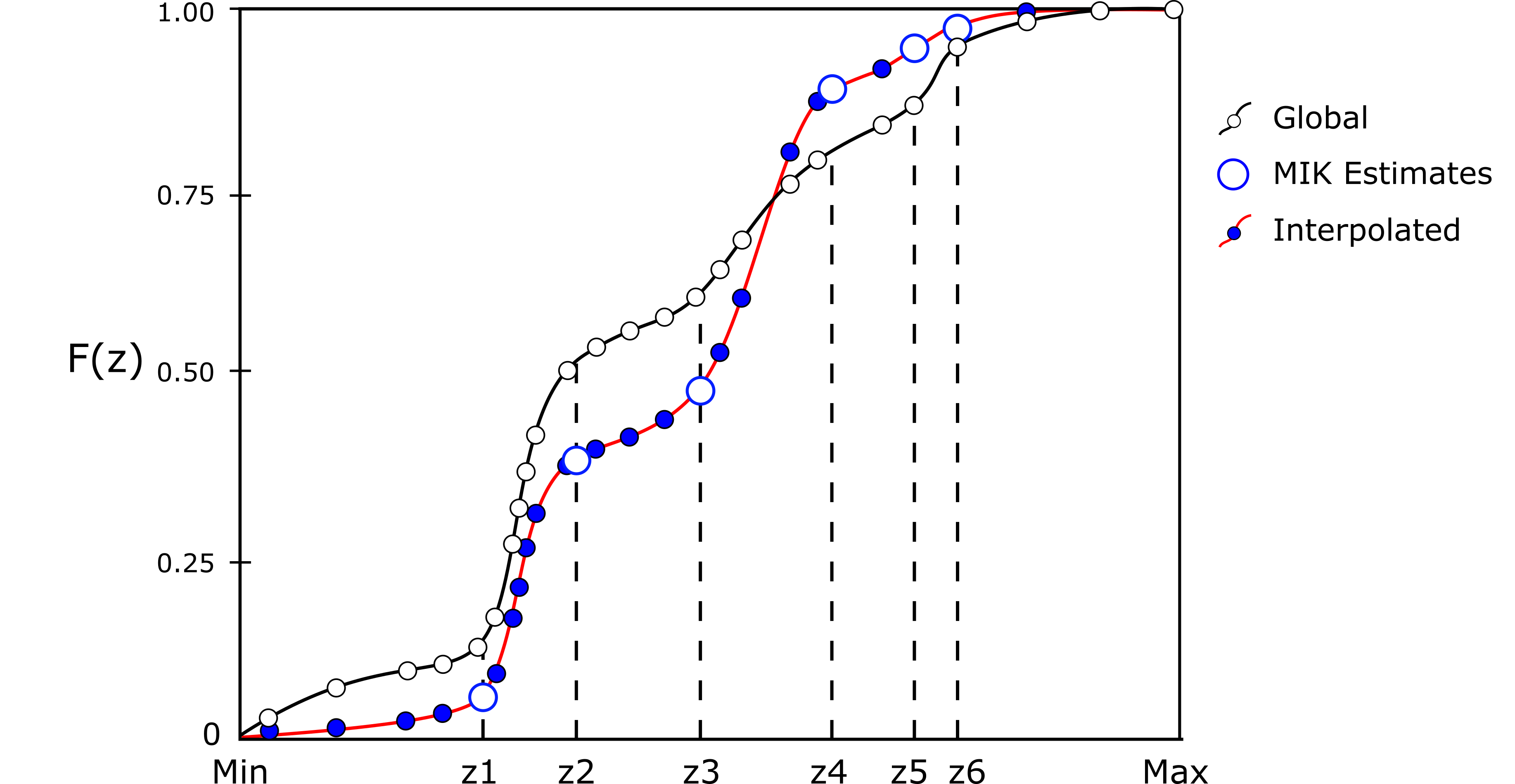
After the order relation correction, it is necessary to interpolate between the estimated CDF values and to extrapolate beyond the first and last thresholds to obtain a complete distribution. Linear, power and hyperbolic models are sometimes used for this step, but in practice it is better to scale the global declustered distribution to fit between the gaps and in the tails. The MIK estimates provide local CDF values at the chosen thresholds for each unsampled location (see blue circles on figure below). The complete local distribution for all \(p\) and \(Z\) values is inferred from these MIK estimates and the global distribution. The shape of the global distribution for each interval is preserved, but scaled to the correct MIK probability estimates and the specified minimum and maximum (see the red dashed line on figure below).
Recoverable Resources
After filling each local distribution, it is possible to obtain any desired summary statistic. These include the mean, variance, other measures of uncertainty, and the probability to be above cutoff. For calculating these statistics, the procedure is to extract \(L\) quantiles (typically 200 in practice) from each filled in non-parametric distribution:
\[z(\textbf{u};l),\quad P_l=\frac{l}{L+1}, \quad l=1,\ldots,L, \quad \textbf{u} \in A \]
So, at each \(\textbf{u}\) each location, there are \(L\) equally spaced quantiles. For block statistics, it is necessary to perform volume support correction from point to block scale. It is common to use the simpler affine or indirect lognormal corrections because there are many distributions to correct. The discrete Gaussian model would be appropriate, but more computationally demanding. The global change of support correction could be applied as a short cut, but the change of support is known to vary locally.
The expected value e-type mean, will be very smooth, but it is a useful summary at each location:
\[ m(\textbf{u}) = \frac{1}{L} \displaystyle\sum_{l=1}^L z(\textbf{u};l), \quad \textbf{u} \in A \]
The variance:
\[ \sigma^2(\textbf{u}) = \frac{1}{L} \displaystyle\sum_{l=1}^L (z(\textbf{u};l)-m(\textbf{u}))^2, \quad \textbf{u} \in A \]
The probability of a block being above some cutoff grade could also be calculated as the number of values above the cutoff grade divided by the total number of values (\(L\)). The grade of the ore is calculated as the average grade of those values above cutoff.
The probability of each block being ore and the grade of ore can be combined for a resource estimate. To estimate the total ore tonnage in a region, it is necessary to sum the product of probability of being ore and the tonnage of the block. The ore grade is the tonnage weighted average of the ore grade of each block. The waste tonnage is the total tonnage minus the ore tonnage.
Considerations
Multiple Indicator Kriging (MIK) is a non-parametric estimation of uncertainty at point scale that makes no explicit assumption about the distribution. This method could be used for complex mineralization, with mixed grade populations that cannot be easily separated in different domains. Other options for probabilistic estimation are the Multi Gaussian methods including Multi-Gaussian Kriging, and Uniform Conditioning.
The block uncertainty provided by MIK could be run through a localization procedure (LIK - Localised Indicator Kriging), to provide a unique value per block that reproduces the block distribution in larger panels (Hardtke, Allen, & Douglas, 2011).
Simulation has many benefits related to joint uncertainty over large volumes and the ability to work with multiple variables. However, MIK/LIK is easy to apply and suitable to situations with complex geological controls on grades.