Learning Objectives

• Review theory of standardized ordinary cokriging with unequally sampled data
• Understand the application and workflow of standardized ordinary cokriging
• Compare results of ordinary kriging to standardized ordinary cokriging

Introduction

Cokriging with unequally sampled data could be used with drill holes (resource and reserve estimation drilling campaigns - exploration data) and blast holes (or other production samples) to improve short- and medium-term models. Both data types complement each other: (1) drill hole data for exploration and estimation stages typically have better quality control than production sampling, and (2) production sampling is more abundant and closely spaced than exploration data. There are many other situations where multiple data types or variables are available at different locations including different vintages of sampling, different drilling types (reverse circulation and diamond drilling) and relatively inexpensive chip or channel samples together with drill hole data.

Cokriging is recommended when the data types are at different locations. This is sometimes referred to as heterotopic data. When multiple variables are measured at the same locations (equally sampled, or homotopic data) kriging can be used to estimate each variable one at the time. Decorrelation techniques can facilitate simulation of homotopic data, techniques like Projection Pursuit Multivariate Transform (Barnett & Deutsch, 2017) have been presented in previous lessons and the reader is encouraged to review them at GeostatisticsLessons.com. Cokriging optimally combines multiple data types accounting for error, bias and different support of the measurements (Minnitt & Deutsch, 2014). This lesson will present standardized ordinary cokriging for drill holes and blast holes. In practice, any number of data types could be considered and the approach could be applied in a non-mining context.

An essential component of cokriging is to have a valid Linear Model of Coregionalization (LMC) for the direct and cross variograms. For the drill hole and blast hole example considered in this Lesson, there are two direct experimental variograms: one for the drill hole data and one for the blast hole data. There is also a cross-covariance between the drill hole and blast hole data. This cross covariance is made to look like a cross variogram for the conventional practice of variogram fitting. In the end, there are three variograms in three directions that must be fit simultaneously for a valid LMC to solve the cokriging equations.

Multiple elements measured in the drill hole and blast hole data will significantly increase the number of variograms required and automatic fitting would be required. In an estimation context, each variable could be considered separately unless they are correlated and one or more are undersampled relative to the rest.

Theory

Consider two variables: (a) Primary variable from exploration data \(\left\{Z\left(\mathbf{u}_{\alpha}\right), \text{where: }\alpha=1, \ldots, n_{Z}\right\}\), and (b) Secondary variable from production sampling: \(\left\{Y\left(\mathbf{u}^{\prime}_{\beta}\right), \text{where: } \beta=1, \ldots, n_{Y}\right\}\). Primary and secondary data will be used to characterize the spatial variability. Both variables are standardized to have a mean of zero and a variance of one by subtracting the mean and dividing by the standard deviation (Rossi & Deutsch, 2013). The stationary domains have been previously defined for different zones of the mineral deposit. The variables are standardized:

\[\begin{equation} \begin{aligned}[c] Z_{std} = \frac{Z\left(\mathbf{u}\right)-m_{Z}}{\sigma_{Z}} \end{aligned} \qquad\qquad \begin{aligned}[c] & Y_{std} = \frac{Y\left(\mathbf{u}\right)-m_{Y}}{\sigma_{Y}} \end{aligned} \end{equation}\]

After the estimation is complete, the values can be back transformed to original units multiplying each estimate by the standard deviation of the primary variable and adding the mean of the primary variable. Care must be taken to have reliable mean and standard deviation values. The direct variograms are denoted:

\[\begin{equation} \begin{aligned} &\gamma_{ZZ}(\mathbf{h})=E\left\{\left[Z{\left(\mathbf{u}\right)}-Z{\left(\mathbf{u}+\mathbf{h}\right)}\right]^{2}\right\} \\ &\gamma_{YY}(\mathbf{h})=E\left\{\left[Y{\left(\mathbf{u}\right)}-Y{\left(\mathbf{u}+\mathbf{h}\right)}\right]^{2}\right\} \\ \end{aligned} \end{equation}\]

The cross variogram and cross covariance are denoted:

\[\begin{equation} \begin{aligned} &\gamma_{ZY}(\mathbf{h})= E\left\{\left[Z{\left(\mathbf{u}\right)}-Z{\left(\mathbf{u}+\mathbf{h}\right)}\right]\left[Y{\left(\mathbf{u}\right)}-Y{\left(\mathbf{u}+\mathbf{h}\right)}\right]\right\}\\ &C_{ZY}(\mathbf{h})=E\left\{Z{\left(\mathbf{u}\right)} Y{\left(\mathbf{u}+\mathbf{h}\right)}\right\}-E\left\{Z{\left(\mathbf{u}\right)}\right\} E\left\{Y{\left(\mathbf{u}+\mathbf{h}\right)}\right\} \end{aligned} \end{equation}\] Under an assumption of first and second-order stationarity, the cross covariance and cross variogram are related: \[\begin{equation} \gamma_{ZY}\left(\mathbf{h}\right) = C_{ZY}\left(\mathbf{0}\right)-C_{ZY}\left(\mathbf{h}\right) \end{equation}\]

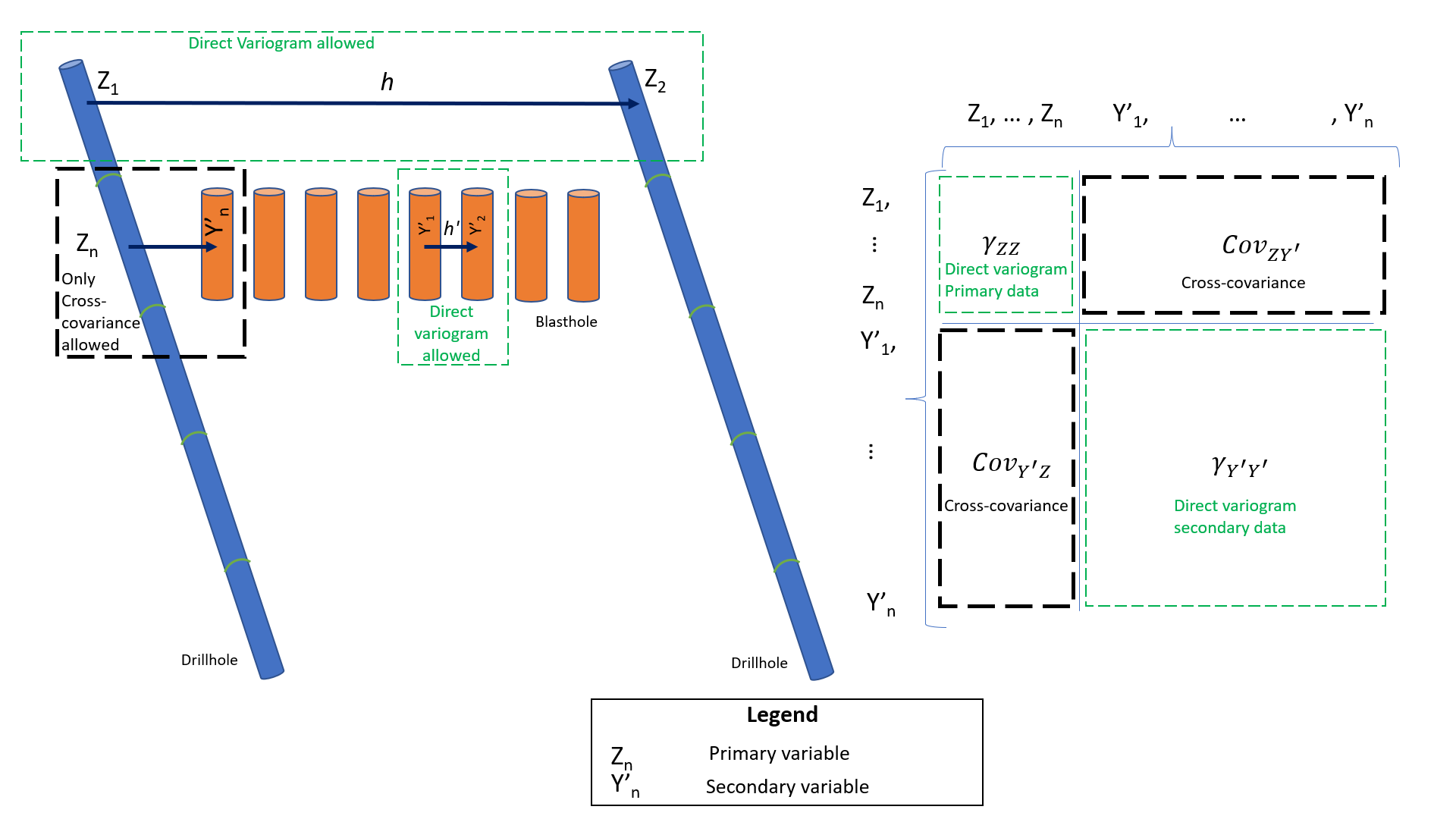
This relationship is very important for heterotopic data because the cross variogram can only be calculated for homotopic data. In practice, the cross covariance is calculated and the cross variogram is then derived from the cross covariance (Donovan, 2015). The cross covariance for a distance of zero (\(C_{ZY}(\mathbf{0})\)) is estimated by extrapolation. Then the cross variogram can be obtained from Equation 4. Cuba and Deutsch give a detailed explanation of this (Cuba & Deutsch, 2012). Figure 1 presents a schematic illustration. For the cross variograms, the presence of both variables (\(Z\) and \(Y\)) is required at both ends of the vector \(\mathbf{h}\), while for the cross covariance, one variable is required at one end and the other variable at the other end. Notice that different data types could have different support, that is, drilling diameter and length of measurement.

The linear model of coregionalization is used to model the three variograms at the same time to ensure that the corresponding covariances are positive definitive (Pyrcz & Deutsch, 2014). The LMC has the following form: \[\begin{equation} \begin{aligned} &\gamma_{\mathrm{ZZ}}(\mathbf{h})=\sum_{l=0}^{n s t} {c}_{\mathrm{ZZ}}^{l} \Gamma_{l}(\mathbf{h}) ={c}_{\mathrm{ZZ}}^{0} +{c}_{\mathrm{ZZ}}^{1}\Gamma_{1}(\mathbf{h}) +{c}_{\mathrm{ZZ}}^{2}\Gamma_{2}(\mathbf{h}) + \ldots \\ &\gamma_{Z Y}(\mathbf{h})=\sum_{l=0}^{n s t} {c}_{Z Y}^{l} \Gamma_{l}(\mathbf{h}) ={c}_{\mathrm{ZY}}^{0} +{c}_{\mathrm{ZY}}^{1}\Gamma_{1}(\mathbf{h}) +{c}_{\mathrm{ZY}}^{2}\Gamma_{2}(h) + \ldots\\ &\gamma_{Y Y}(\mathbf{h})=\sum_{l=0}^{n s t} {c}_{Y Y}^{l} \Gamma_{l}(\mathbf{h}) ={c}_{\mathrm{YY}}^{0} +{c}_{\mathrm{YY}}^{1}\Gamma_{1}(\mathbf{h}) +{c}_{\mathrm{YY}}^{2}\Gamma_{2}(h) + \ldots \\ \end{aligned} \end{equation}\]

Where: \(nst\) is the number of structures; \({c}_{\mathrm{ZZ}}^{l}\) are the contributions for the \(l\) structures; and, \(\Gamma_{l}(\mathbf{h})\) are the variograms of the \(l\) nested structures. The contribution coefficients (\({c}_{\mathrm{ZZ}}^{l}\)) could be different for each model as long they meet the following conditions to ensure a positive definite valid variogram model (Pyrcz & Deutsch, 2014):

\[\begin{equation} \begin{aligned}[c] & {c}_{\mathrm{ZZ}}^{l}>0\\ & {c}_{\mathrm{YY}}^{l}>0\\ & {c}_{\mathrm{ZZ}}^{l}\cdot{c}_{\mathrm{YY}}^{l}\ge{c}_{\mathrm{ZY}}^{l}\cdot{c}_{\mathrm{ZY}}^{l}\\ \end{aligned} \qquad\qquad \begin{aligned}[c] & \forall \; l \end{aligned} \end{equation}\] Now, the standardized ordinary cokriging estimator can be written as (Minnitt & Deutsch, 2014): \[\begin{equation} \begin{aligned} \frac{Z_{S O C K}^{*}\left(\mathbf{u}_{0}\right)-m_{Z}}{\sigma_{Z}}=\sum_{\alpha=1}^{n_{Z}} \lambda_{\alpha {\left(\mathbf{u}_{0}\right)}}\left[\frac{Z\left(\mathbf{u}_{\alpha}\right)-m_{Z}}{\sigma_{Z}}\right]+ \sum_{\beta=1}^{n_{Y}} \lambda_{\beta \left(\mathbf{u}_{0}\right)}^{\prime}\left[\frac{Y\left(\mathbf{u}^{\prime}_{\beta}\right)-m_{Y}}{\sigma_{Y}}\right]\ \end{aligned} \end{equation}\]\end{equation} Where \(\lambda_{\alpha \left(\mathbf{u}_{0}\right)}\) and \(\lambda^{\prime}_{\beta \left(\mathbf{u}_{0}\right)}\) are the cokriging weights for the primary variable and the secondary variable, respectively at location \(\mathbf{u}_{0}\); \(m_{z}=E\{Z(\mathbf{u})\}\) and \(m_{y}=E\{Y(\mathbf{u})\}\) are the stationary means of \(Z\) and \(Y\) respectively; \({n_{Z}}\) and \({n_{Y}}\) are the number of samples inside the ranges of influence of the variogram (or covariance) for the primary and secondary variable, respectively. There is only one condition in order to get an estimator that is unbiased (Isaaks & Srivastava, 1989 ; Deutsch & Journel, 1997): \[\begin{equation} \sum_{\alpha=1}^{n_{Z}} \lambda_{\alpha \left(\mathbf{u}_{0}\right)}+\sum_{\beta=1}^{n_{Y}} \lambda_{\beta \left(\mathbf{u}_{0}\right)}^{\prime}=1 \end{equation}\]

Some historical implementations of ordinary cokriging considered the condition that the sum of the weights to the secondary data should be zero. This is a severe constraint that undermines the improvement brought by cokriging (Deutsch & Journel, 1997 ; Minnitt & Deutsch, 2014). A single constraint ensures that the secondary data are weighted appropriately (Goovaerts, 1998). Minimizing the mean squared error (MSE) generates the cokriging system of equations. Since there is only one constraint (see Equation 8) there is one Lagrange parameter. The system of equations:

\[\begin{equation} \begin{aligned} &\sum_{i=1}^{n_{Z}} \lambda_{i \left(\mathbf{u}_{0}\right)} C_{Z Z}\left(\mathbf{u}_{\alpha}-\mathbf{u}_{i}\right)+\sum_{j=1}^{n_{Y}} \lambda_{j \left(\mathbf{u}_{0}\right)}^{\prime} C_{Z Y}\left(\mathbf{u}_{\alpha}-\mathbf{u}_{j}^{\prime}\right) +\mu_{\left(\mathbf{u}_{0}\right)}=C_{Z Z}\left(\mathbf{u}_{\alpha}-\mathbf{u}_{0}\right) \quad \\ &\text{where } \alpha=1, \ldots, n_{Z \left(\mathbf{u}_{0}\right)} \\ &\sum_{i=1}^{n_{Z}} \lambda_{i \left(\mathbf{u}_{0}\right)} C_{Y Z}\left(\mathbf{u}_{\beta}^{\prime}-\mathbf{u}_{i}\right)+\sum_{j=1}^{n_{Y}} \lambda_{j \left(\mathbf{u}_{0}\right)}^{\prime} C_{Y Y}\left(\mathbf{u}_{\beta}^{\prime}-\mathbf{u}_{j}^{\prime}\right)+\mu_{\left(\mathbf{u}_{0}\right)}=C_{Y Z}\left(\mathbf{u}_{\beta}^{\prime}-\mathbf{u}_{0}\right) \quad \\ &\text{where } \beta=1, \ldots, n_{Y \left(\mathbf{u}_{0}\right)} \\ & \sum_{\alpha=1}^{n_{Z}} \lambda_{i \left(\mathbf{u}_{0}\right)}+\sum_{\beta=1}^{n_{Y}} \lambda_{j \left(\mathbf{u}_{0}\right)}^{\prime}=1 \end{aligned} \end{equation}\]

This can be expressed in matrix form as:

\[\begin{equation} \begin{bmatrix} C_{ZZ}(\mathbf{u}_1 - \mathbf{u}_1) & \ldots & C_{ZZ}(\mathbf{u}_1 - \mathbf{u}_{n_{Z}}) & C_{ZY}(\mathbf{u}_1 - \mathbf{u}^{\prime}_1) & \ldots & C_{ZY}(\mathbf{u}_1 - \mathbf{u}^{\prime}_{n_{Y}}) & 1\\ \vdots & \ddots & \vdots & \vdots & \ddots & \vdots\\ C_{ZZ}(\mathbf{u}_{n_{Z}} - \mathbf{u}_1) & \ldots & C_{ZZ}(\mathbf{u}_{n_{Z}} - \mathbf{u}_{n_{Z}}) & C_{ZY}(\mathbf{u}_{n_{Z}} - \mathbf{u}^{\prime}_1) & \ldots & C_{ZY}(\mathbf{u}_{n_{Z}} - \mathbf{u}^{\prime}_{n_{Y}}) & 1 \\ C_{YZ}(\mathbf{u}^{\prime}_1 - \mathbf{u}_1) & \ldots & C_{YZ}(\mathbf{u}^{\prime}_1 - \mathbf{u}_{n_{Z}}) & C_{YY}(\mathbf{u}^{\prime}_1 - \mathbf{u}^{\prime}_1) & \ldots & C_{YY}(\mathbf{u}^{\prime}_1 - \mathbf{u}^{\prime}_{n_{Y}}) & 1\\ \vdots & \ddots & \vdots & \vdots & \ddots & \vdots\\ C_{YZ}(\mathbf{u}^{\prime}_{n_{Y}} - \mathbf{u}_1) & \ldots & C_{YZ}(\mathbf{u}^{\prime}_{n_{Y}} - \mathbf{u}_n) & C_{YY}(\mathbf{u}^{\prime}_{n_{Y}} - \mathbf{u}^{\prime}_1) & \ldots & C_{YY}(\mathbf{u}^{\prime}_{n_{Y}} - \mathbf{u}^{\prime}_{n_{Y}}) & 1\\ 1 & \ldots & 1 & 1 & \ldots & 1 & 0 \\ \end{bmatrix} % \begin{bmatrix} \lambda_1 \\ \vdots \\ \lambda_{n_Z} \\ \lambda^{\prime}_1 \\ \vdots \\ \lambda^{\prime}_{n_Y}\\ \mu\\ \end{bmatrix} \\ = \begin{bmatrix} C_{ZZ}(\mathbf{u}_1 - \mathbf{u}_0) \\ \vdots\\ C_{ZZ}(\mathbf{u}_n - \mathbf{u}_0) \\ C_{YZ}(\mathbf{u}^{\prime}_1 - \mathbf{u}_0) \\ \vdots\\ C_{YZ}(\mathbf{u}^{\prime}_n - \mathbf{u}_0) \\ 1\\ \end{bmatrix} \end{equation}\]

Since weights are calculated for each location being estimated, a consistent notation would be \(\lambda_1(\mathbf{u}_0)\) instead of \(\lambda_1\) (as in Equation 9), nevertheless, for the matrix form, the latter is being used because of space.

The cokriging estimator of Equation 7 will account for bias through the different mean values and account for error and different support through the covariance values. This estimator could be used directly in short- or medium-term modeling. In the case of simulation, the use of simple cokriging would be recommended to be consistent with the multivariate Gaussian distribution. This Lesson is aimed at estimation.

Implementation

The first step is to perform an exploratory data analysis to recognize the different characteristics of the data. Care should be taken if the information comes from different laboratories. The data are commonly processed separately within different domains. Basic statistics and visualization of the data are minimum steps. The next step is to standardize both data types by subtracting the mean and dividing by the standard deviation for each value. There will be different mean and standard deviation values for each data type.

The principal directions of continuity (major, minor and tertiary) are identified and defined. Experimental variograms of the drill holes and blast holes are calculated with different distance and direction tolerances since the data are spaced differently. The cross-covariance can be calculated with its own tolerance parameters, however, the value at \(\mathbf{h}=0\) (\(C(0)\)) will be inferred from the experimental model of the covariance. The cross variogram is then inferred.

The three experimental variograms are modeled at the same time with the LMC. The same models and structures are used with different contributions. The practitioner can consider the direct variogram of drill holes as first priority, then the cross variogram and finally the direct variogram of the blast holes. Once the variograms have been modeled, the cokriging program can be used. It is useful to perform ordinary kriging with the primary data only to ensure that the cokriging is performing well, the results of cross-validation can be assessed.

Example

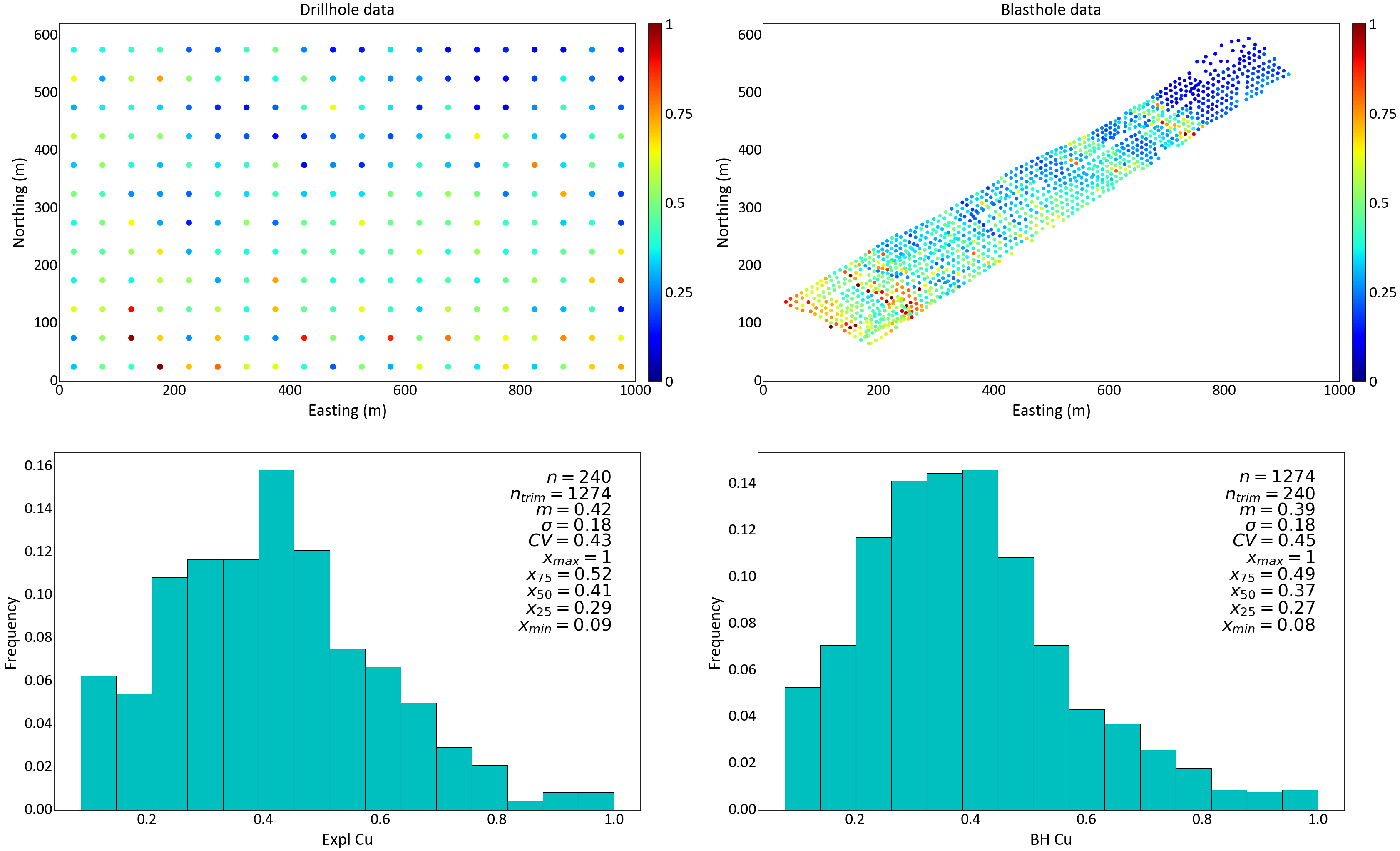
A set of copper values from exploration data (drill holes) and production data (blast holes) are considered. The location of the data and summary statistics and histograms are presented in Figure 2. As a detail, the file to be used with the GSLIB program ‘cokb3d’ should contain both data types, one column with exploration data and another column with production data, this implies that half of the data entries will be missing values. Then, it is necessary to standardize both data types.

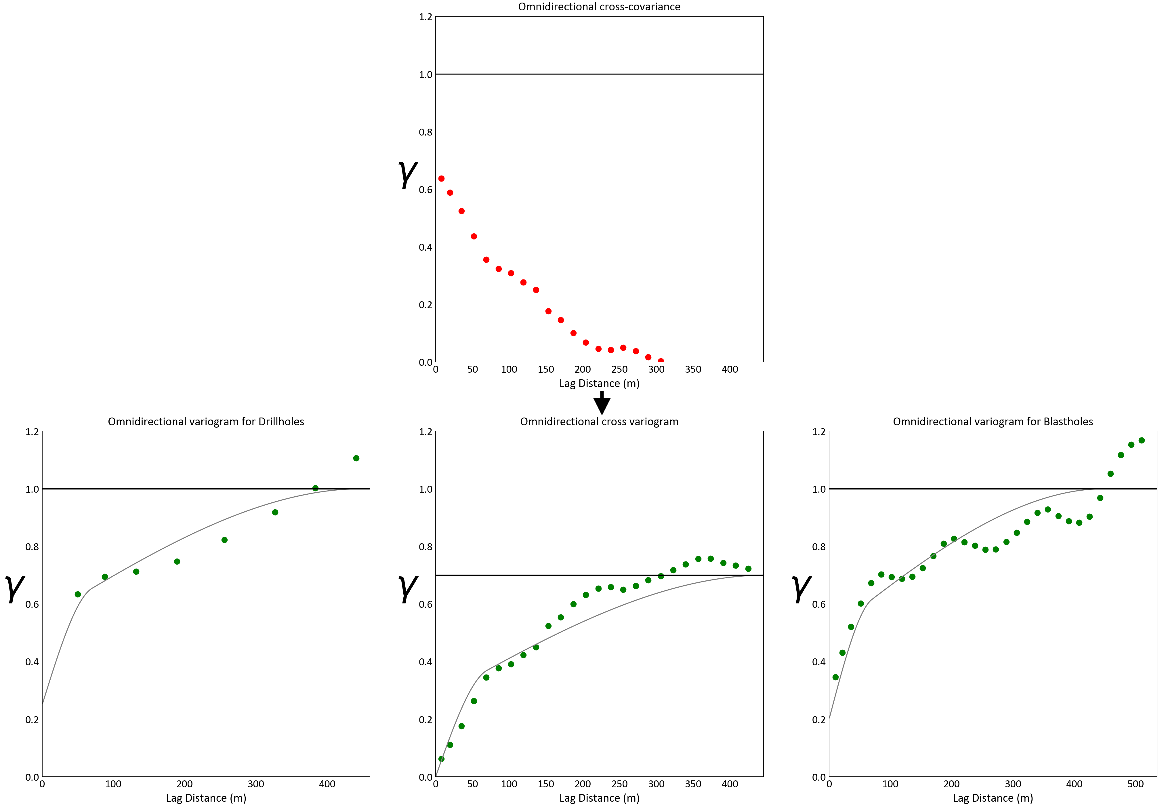
The next step is to find the major directions of continuity. In this example an omnidirectional variogram is used, although anisotropy can be recognized in blast hole data (major direction: N 120, minor direction N 30); however, it cannot be clearly recognized in the drill hole data. Figure 3 shows the calculation of the experimental variograms and its models. The cross-covariance was calculated first and used to derive the cross-variogram. The three experimental variograms are modeled at the same time, only the contributions of each structure for every variogram model can be different (see Equation 5). The model is checked to ensure it is positive definitive (see Equation 6). A spherical model is used, the LMC is shown:

\[\begin{eqnarray} \nonumber \gamma_{ZZ}\left( \mathbf{h} \right) &=& 0.25 \; \textrm{Nugget} + 0.30 \; \textrm{Sph}_{a=70} \left( \mathbf{h} \right) + 0.45 \; \textrm{Sph}_{a=450} \left( \mathbf{h} \right) \\ \nonumber \gamma_{YZ}\left( \mathbf{h} \right) &=& 0.00 \; \textrm{Nugget} + 0.27 \; \textrm{Sph}_{a=70} \left( \mathbf{h} \right) + 0.43 \; \textrm{Sph}_{a=450} \left( \mathbf{h} \right) \\ \nonumber \gamma_{YY}\left( \mathbf{h} \right) &=& 0.20 \; \textrm{Nugget} + 0.30 \; \textrm{Sph}_{a=70} \left( \mathbf{h} \right) + 0.50 \; \textrm{Sph}_{a=450} \left( \mathbf{h} \right) \end{eqnarray}\]

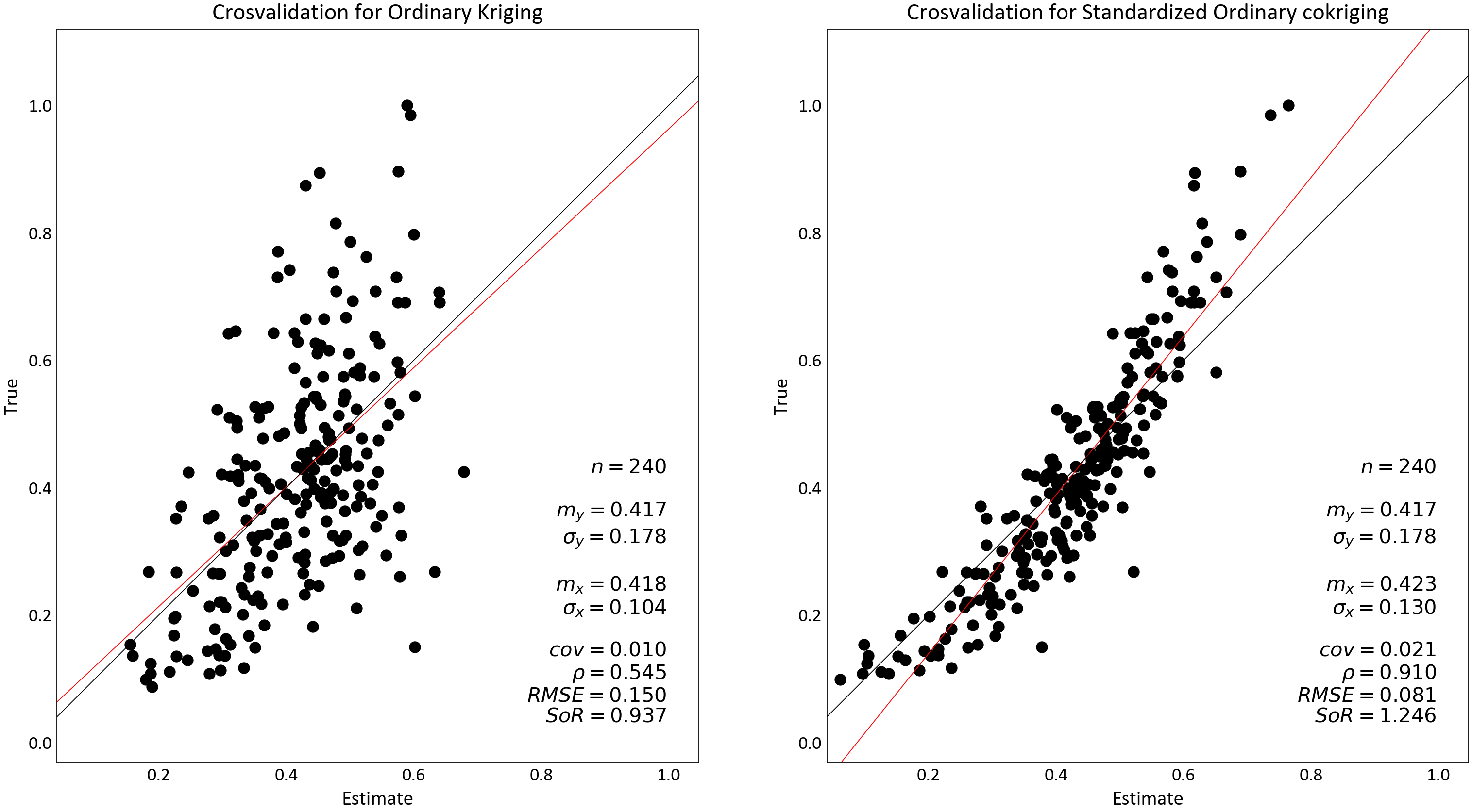
Ordinary kriging and standardized ordinary cokriging are performed to obtain estimates in original units. Cross validation results are shown. The fit for kriging is reasonably good; however, the fit for cokriging is better. Maps of both estimates are displayed with subtle, yet important, local changes in the area of the blast holes that shows a better definition of grades.

Discussion

Theoretically, cokriging with more information should always perform better than kriging. This is shown in the example. The good results depend on reasonable variogram fitting and a reasonable assessment of the blast hole data. The main application of the methodology presented, in mining geostatistics applications, will be short- and medium term modeling. There are similar applications in environmental geostatistics with data of different quality. An important outstanding topic is simulation and the assessment of uncertainty with multiple data types. This is an evident extension of the theory and example presented here, but not developed in this lesson. Another related topic is the possibility of using data imputation instead of cokriging, that is, impute the true values given collocated measured values with error. This imputation approach would be suited to simulation.

Summary

Standardized ordinary cokriging (SOCK) is a useful tool to apply in mining with higher quality exploration data and short term production data. The cross variogram of heterotopic data cannot be directly obtained; however, the cross covariance can be used as an estimator. The LMC must be positive definitive and all variograms are fitted simultaneously. The final cokriging outperforms ordinary kriging.

References