Cite this lesson as: Samson, M., Deutsch, C.V. (2021). The Sill of the Variogram. In J. L. Deutsch (Ed.), Geostatistics Lessons. Retrieved from http://www.geostatisticslessons.com/lessons/sillofvariogram
The Sill of the Variogram
Matthew Samson
University of Alberta
Clayton V. Deutsch
University of Alberta
August 17, 2021
Learning Objectives
- Review variogram modeling and key parameters including the sill
- Understand when to model the variogram above the sill
- Demonstrate how careful variogram modeling improves estimation
Introduction
The variogram is a key input to change of support, kriging, and simulation. It is partly data-driven from experimental variogram points calculated from the available data and partly model-driven from the experience of the geostatistician and geological analogues; the variogram model fits the experimental points and incorporates general knowledge. The variogram is defined with relatively few parameters. The nugget effect, range and sill are common descriptive terms and specific parameters in a variogram model. The sill is the focus of this Lesson.
There are many excellent references in geostatistics that discuss the variogram at length. Some classics include Cressie (2015), Goovaerts (1997), Chiles & Delfiner (2009), and Rossi & Deutsch (2014). The Teacher’s Aide Gringarten & Deutsch (2001) is another good reference.
The sill is commonly considered to be the variogram value where the variogram points or function flatten off at increasing distance; however, the variogram may not flatten off in some directions and it may flatten off at different values in different directions. The sill may also be considered as the limit of the variogram as the lag distance tends to infinity. The sill is also considered to be the variance of the data entering variogram calculation, but we still face questions about how to model the variogram relative to the variance. Recommendations for this are provided below.
English words usually have a different meaning depending on context. Our definition of Variogram Sill in geostatistics: 1. the horizontal variance level where the variogram flattens off (as a descriptive value); 2. the variance of the data used in variogram calculation (for interpretation - variogram values below this are directly related and values above this are inversely related); 3. the sum of variance contributions in a variogram model of a stationary regionalized variable (as a parameter of the variogram model).
Variogram
Spatial variability is quantified with a variogram. Consider a regionalized variable within a deemed stationary domain \(\{Z(\textbf{u}), \textbf{u} \in A\}\) where \(Z\) denotes the variable, \(\textbf{u}\) denotes location and \(A\) denotes the domain. The variogram is defined as:
\[ 2{\gamma}(\mathbf{h}) = E \{ [Z(\mathbf{u}) - Z(\mathbf{u}+\mathbf{h})]^2 \} \]
where \(\mathbf{h}\) is a lag vector. \(\gamma\) is technically the semivariogram, but we refer to it as the variogram hereafter. The experimental variogram \(\hat{\gamma}\) is computed for direction and distance lags as possible:
\[ \hat{\gamma}(\textbf{h}) = \frac{1}{2N(\textbf{h})} \sum_{i=1}^{N(\textbf{h})} [Z(\mathbf{u_i}) - Z(\mathbf{u_i+h})]^2 \]
where \(N(\textbf{h})\) pairs of samples are separated approximately by the lag vector \(\textbf{h}\). Calculating reliable variograms in appropriate directions are the subjects of other Lessons. The experimental variograms shown as the colored dots in the figure below are interesting. The directional variograms (two horizontal on the left and vertical on the right) are standardized so the sill (definition 2) is 1.0. According to definition 1, the sills for the horizontal variograms are 0.55 and 0.8; the sill for the vertical is aiming toward a value above 1.4. These variograms were modeled by the solid lines - they all have a sill of 1.0.

The experimental variogram values are supplemented by general geological knowledge and the variogram is modeled by a valid function. Geostatistical calculations require the variogram for distances and directions that are not reliably informed from the available data Also, the variogram must constitute a valid measure of distance in the kriging equations. The form of almost all variogram modeling is taken from the Linear Model of Regionalization (LMR), that is, a sum of nested structures:
\[ \gamma(\mathbf{h}) = \sum_{i=0}^{nst} c_{i}\Gamma_{i}(\mathbf{h}) \]
\(\Gamma^{i}(\mathbf{h})\) are the pool of \(i = 0,\ldots,nst\) structures, where the \(0^{th}\) nested structure is the nugget effect by convention, \(c_i\) is the contribution of the \(i^{th}\) structure, and each structural variogram (\(i = 1,\ldots,nst\)) is defined by seven parameters - three angles and three ranges (that define anisotropy) and a shape (often spherical, exponential or Gaussian). The variogram value can be calculated in any direction from this equation. If second order stationarity is defined, then the covariance is calculated from the variogram:
\[ C (\mathbf{h}) = \sigma^2 - \gamma_{z}(\mathbf{h}) \]
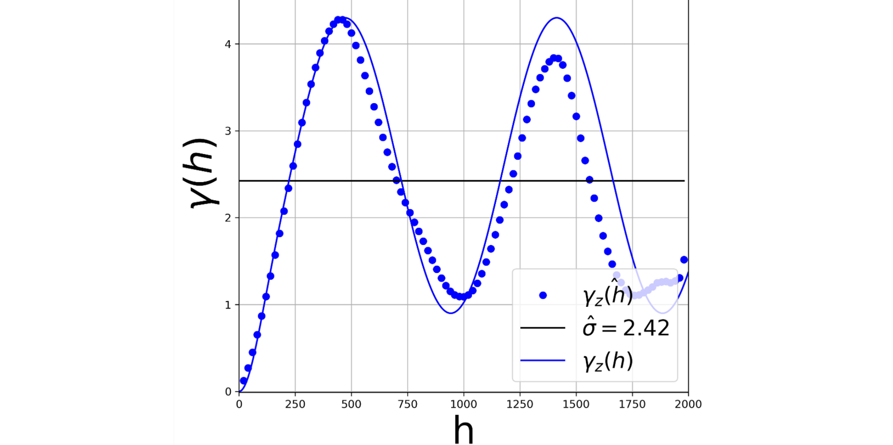
where \(\sigma^2\) is the variance or 1.0 if standardized (Rossi & Deutsch (2014)). There are some important questions outstanding in our discussion of the sill:- What do we do about cyclical variograms that oscillate above and below the variance? The figure below shows an example where the variance is 2.42 and the variogram goes above that (over 4.0) and back below (to nearly 1.0).
- What variance is used for variogram standardization or the sill - declustered or equal weighted?
- Should the variogram model be limited to the expected variance sill or match the data?

The variogram model enters kriging and simulation - the experimentally calculated points do not. Getting the variogram model right is important. Conventional wisdom would tell us to fit the variogram at a short scale; this portion of the variogram will significantly influence estimates and simulated values. In the next section, the kriging equations will be discussed, the effects of fitting the variogram above the variance will be discussed.
Kriging
Simple kriging (SK) is widely used in the context of the multivariate Gaussian distribution for simulation and conditioning. Ordinary kriging (OK) is widely used for block modeling for resource estimation. The SK estimator is written as:
\[ z({\mathbf u}_0)_{SK}-m=\sum^n_{i=1} \lambda_{SK,i} \cdot \left [z({\mathbf u}_i) - m \right ] \]
where \(z({\mathbf u}_0)^*\) is the estimator at the unsampled location, \(m\) is the mean, \(z({\mathbf u}_i),i=1,\ldots,n\) are the data and \(\lambda_{SK,i},i=1,\ldots,n\) are the weights applied to the data. The weights are calculated to minimize the expected error variance; they are solved assuming the stationary covariance between the data and between the data and unsampled location come from \(C (\mathbf{h}) = \sigma^2 - \gamma_{z}(\mathbf{h})\):
\[ \sum^n_{j=1} \lambda_{SK,j} C (\mathbf{u}_i - \mathbf{u}_j) = C (\mathbf{u}_0 - \mathbf{u}_i) \qquad i = 1,\ldots,n \]
The OK estimator is written without the mean and is widely recognized as a more robust estimator in kriging for resource estimation. It is also more flexible to control the smoothing of the final estimate. The OK estimator:
\[ z({\mathbf u}_0)_{OK}=\sum^n_{i=1} \lambda_{OK,i} \cdot z({\mathbf u}_i) \]
where \(\lambda_{OK,i},i=1,\ldots,n\) are the OK weights applied to the data. These weights are solved using a pseudo covariance between the data and between the data and unsampled location coming from \(C (\mathbf{h}) = C_{max} - \gamma_{z}(\mathbf{h})\) where \(C_{max}\) could be the variance, but is often the sum of variance contributions in the variogram model:
\[ \left\{\begin{matrix} \sum^n_{j=1}\lambda_{OK,j} \cdot C (\mathbf{u}_i - \mathbf{u}_j) +\mu = C (\mathbf{u}_0 - \mathbf{u}_i) \qquad i = 1,...,n \\ \sum^n_{j=1}\lambda_{OK,j} = 1 \end{matrix}\right. \]
Many sources of confusion in the sill can now be summarized.
- For a stationary regionalized variable, the variance should be used for both SK and OK to compute the covariance to enter the kriging equations.
- The variance used in converting the variogram to covariance values should be the variance considered in the variogram calculation or in the standardization of the variogram - the equal weighted variance since the pairs are almost always equally weighted. Variogram declustering would be considered on a case-by-case basis since there are different formalisms for that.
- For a stationary regionalized variable, the sum of variance contributions should equal the variance.
- For a non-stationary or cyclical regionalized variable the sum of variance contributions in variogram modeling will not be the variance. The sum of variance contributions should not be used in SK with a non-stationary variogram; the variance should be used.
- For OK with a non-stationary variogram, the \(C_{max}\) could be either the variance or the sum of variance contributions. The weights will be the same in both cases.
Suboptimal results will be obtained when the variogram of a stationary variable is not fit to the variance. Suboptimal results may be obtained with SK if the software assumes that the sum of variance contributions is equal to the variance. The first case can be managed by the professional practice. The second case may require checking the software. Unfortunately, the GSLIB software Deutsch & Journel (1998) assumes the sum of variance contributions is the variance. The code should be modified or the variogram sill fitted to the variance for SK in presence of a trend or cyclicity.
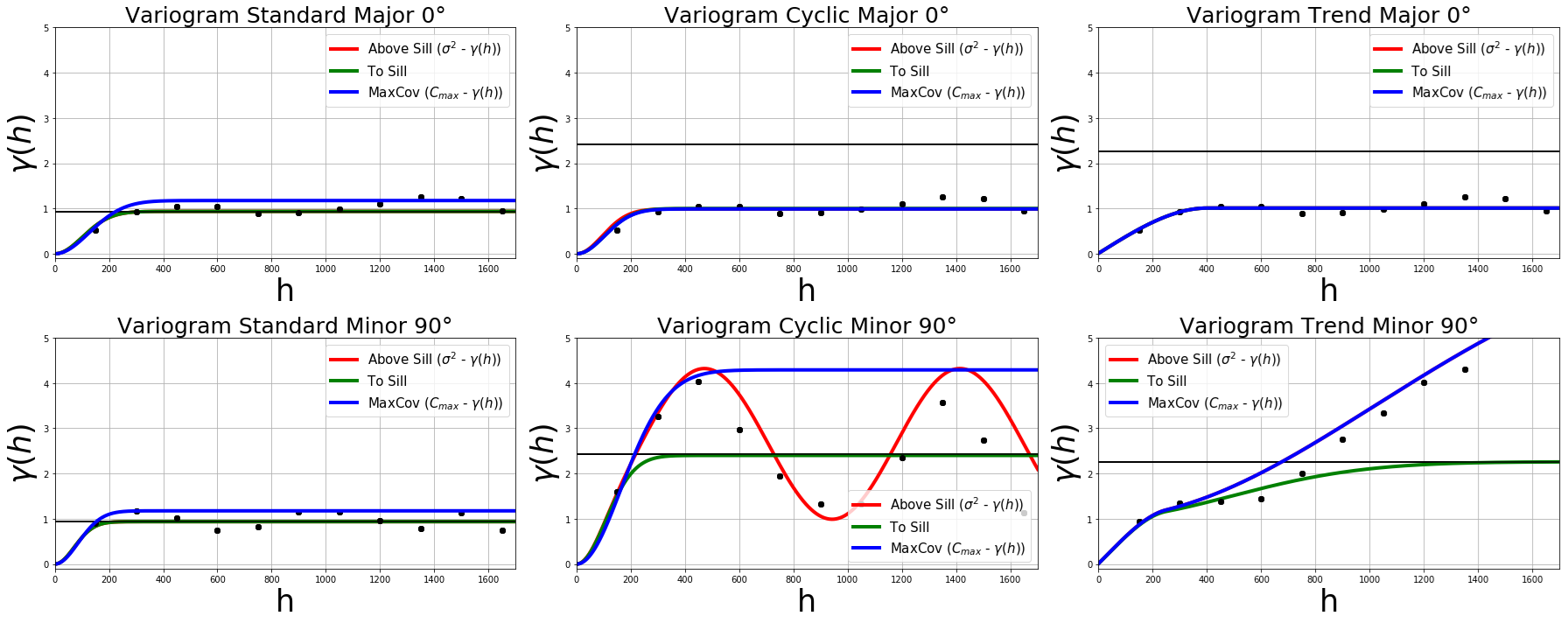
The three options of modeling the variogram are Above The Sill where the variogram is modeled to the experimental points, but the correct variance is used in the covariance calculation, To The Sill” where the variogram is modeled to the variance and the variance is used in the covariance calculation, and MaxCov as Sill* where the variogram is modeled to the experimental points and the sum of variance contributions is used in the covariance calculation. These are illustrated in the sketch below.

A number of validation runs were performed on real and synthetic data to confirm the recommendations described above. The table below summarizes one set of results for two dimensional data with a reasonable data spacing. The three data sets were simulated: Standard corresponds to a stationary variable, Cyclic corresponds to a variable that shows a pronounced cyclicity in one direction, and Trend corresponds to a variable with a pronounced trend in one direction. The performance varies depending on the case, but the improvement for modeling the variogram and managing the sill correctly is likely between 1% to 3% in practice. This is significant.


In summary, the variogram should be fit to reliably calculated variogram points (above or below the sill) and the variance should be used in the covariance calculation. Note that this is not standard practice in all software.
Conclusion
The sill is an important variogram parameter that is defined and used differently in different contexts. This Lesson clarifies that the sill is a qualitative term describing where the variogram flattens off, a specific value equal to the variance of the data entering variogram calculation and a specific value equal to the sum of variance contributions in the conventional modeling of a variogram with the linear model of regionalization. The sum of variance contributions should be set to the variance for stationary simple kriging (SK). The sum could differ from the variance in specific instances; however, the variance should be specified separately and used correctly to transform the variogram values to covariance values. Ordinary kriging (OK) is more robust with respect to how the variogram is fitted since a pseudo-covariance is used in the solution of the OK equations.