Learning Objectives

• Review the importance of categorical variable simulation
• Understand Sequential Indicator Simulation
• Appreciate how secondary information reduces uncertainty

Introduction

Sequential Indicator Simulation (SIS) is a variogram-based categorical simulation technique developed by André Journel and François Alabert (Alabert, 1987). It is implemented in most commercial software for geostatistical modeling. SIS is appropriate when there is no clear geological body geometry, and the spatial continuity is well described by variograms, for example, in highly diagenetically altered facies (Pyrcz & Deutsch, 2014). Over the years, several authors (Deutsch, Journel, et al., 1992; Gómez-Hernández & Srivastava, 1990; P. Goovaerts, 1994; Pierre Goovaerts et al., 1997) implemented SIS with modifications related to various estimators and the use of secondary variables. Deutsch (2006) combined these variations in a GSLIB-like (Deutsch et al., 1992) software. This lesson uses a version of that program to demonstrate the application of SIS.

Conditional simulation generates equiprobable realizations that honor a pre-defined structure and the data inputs. Each realization is a possible outcome of the random function. Kriging minimizes the estimation variance leading to smooth spatial models. Simulation preserves the variability; therefore, it should be used when variability is critical to the result (A. Journel & Isaaks, 1984). Variations in permeability have a large influence on the predicted flow response; therefore, simulation is preferred in most petroleum reservoir characterization. Simulation often follows a sequential random path that ensures the resulting realizations reproduce the data, univariate and bivariate statistics (Pyrcz & Deutsch, 2014).

Categorical variables

Categorical variables are discrete variables defined through a description, name or label. In geological modeling the most common type of categorical variable is based on facies or rock type considering different depositional or alteration characteristics. They have a central role in establishing volumes within which continuous variables are considered stationary (Deutsch, 2006). For example, porosity can change abruptly from floodplain sediments to fluvial channels. In that case, a facies model improves the continuous rock property distribution, helping to define different stationary domains based on geological concepts.

Consider a set of mutually exclusive categories indexed by \(k = 1,\ldots,K\). Indicators (A. G. Journel, 1983) represent the probability of a given category k being present at a location, that is, when the indicator is 1, the category is present and when it is 0, the category is not present. A constant discretization length is common practice. \[ i({\mathbf u} ; k ) = \left\{ \begin{array}{ll} 1, & \mbox{if category } \; k \;\mbox{ prevails at location } {\mathbf u} \\ 0, & \mbox{otherwise} \end{array} \right.,k=1,\ldots,K. \]

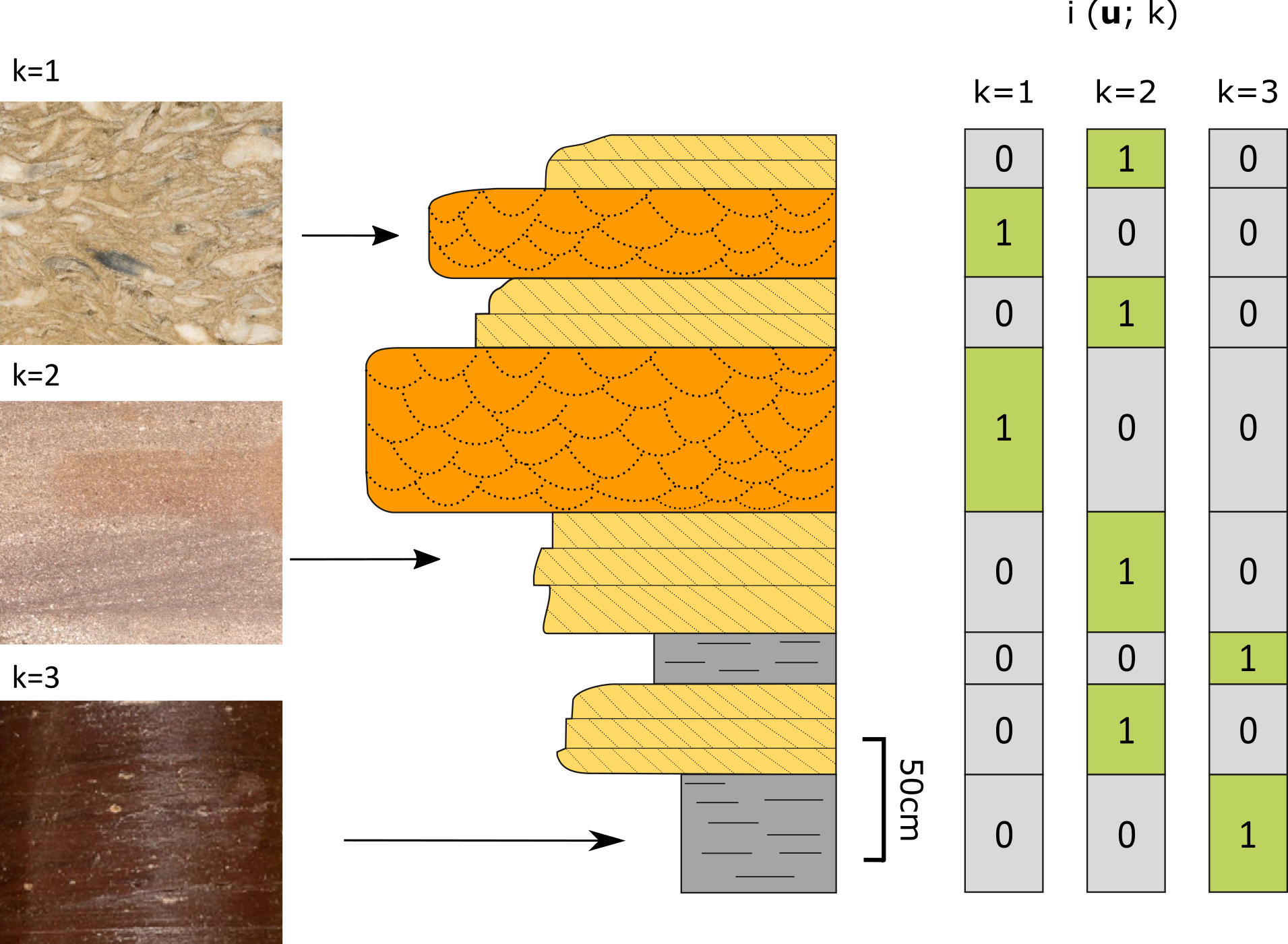
The mean of an indicator variable \(\hat{p}_k\) (Pyrcz & Deutsch, 2014) is the proportion of the category. The mean with declustering weights \(w_j\) is given by: \[ \hat{p}_k = \sum_{j = 1}^{N}w_ji({\mathbf u}_j;k) \]

In addition, the variance is a function of the mean:

\[ \widehat{Var}\{i({\mathbf u};k)\} = \sum_{j = 1}^{N} w_j \; \cdot \; [i({\mathbf u}_j;k) -\hat{p}_k]^2 \] \[ = \hat{p}_k (1.0 - \hat{p}_k) \] The univariate statistics are important, but the spatial statistics are key to define uncertainty and heterogeneity. Experimental variograms are calculated from the indicators (Deutsch et al., 1992): \[ \hat{\gamma}({\mathbf h})_k = \frac{1}{2N({\mathbf h})} \sum\limits_{N({\mathbf h})} [i({\mathbf u};k)- i({\mathbf u} + {\mathbf h};k)]^2, \;\;\; k=1,...,K. \] Indicators have linear increments, thus only linear models like spherical and exponential are allowed, that is, a Gaussian variogram cannot apply to indicator variables. The size of the facies intervals should be large relative to the block size or discretization interval; therefore, the nugget effect on the indicator variograms should be zero. If the size of the intervals are small relative to the block size, then there would be mixing within the blocks and the concept of a categorical variable becomes invalid.

The indicator variograms should be modeled consistently, that is, they are not independent since the indicators for multiple facies are coregionalized in the same space. There is no check for this, but fitting all experimental variograms carefully will mitigate problems with the indicator estimates.

Indicator kriging

There is no explicit random function model for indicators. Local conditional probability distributions are estimated by kriging. The best kriging option will depend on the stationarity decision and the use of secondary data. The BlockSIS (Deutsch, 2006) program implements nine kriging options to estimate the probabilities. This lesson covers the three most relevant options: stationary simple kriging (SK), ordinary kriging (OK), and nonstationary simple kriging using residuals from a locally varying mean (LVM).

Stationary simple kriging estimates the probability for each category based on the conditioning data and a declustered global mean value. There is no use of secondary variables. The estimator is defined as:

\[ i_{SK}^*({\mathbf u};k) - \hat{p}_k = \sum_{\alpha = 1}^{n} \lambda^{SK}_\alpha ({\mathbf u};k) \cdot [i({\mathbf u}_\alpha ;k) - \hat{p}_k]\]

In ordinary kriging, the sum of the weights is constrained to one so that the global mean receives no weight; the sample data receive all the weight. The estimator is defined as:

\[ i_{OK}^*({\mathbf u};k) =\sum_{\alpha = 1}^{n} \lambda_{\alpha}^{OK} ({\mathbf u};k) \cdot i({\mathbf u}_\alpha ;k) \]

Nonstationary simple kriging with locally varying means calculates the weights in the same way as stationary simple kriging, with locally varying mean values at every location. A trend or secondary data define the local probabilities. The estimator is written as:

\[ i_{LVM}^*({\mathbf u};k) - p_k({\mathbf u}) =\sum_{\alpha = 1}^{n} \lambda_{\alpha}^{SK} ({\mathbf u};k) \cdot [i({\mathbf u}_\alpha;k) - p_k({\mathbf u}_\alpha)]\]

Indicator kriging is repeated for each category considering the category-specific variogram.

Kriging can lead to negative weights applied to data screened behind closer samples. In general, this facilitates local extrapolation and can improve the estimation; however, in some cases, depending on the variogram and local data configuration, this could lead to negative indicator estimates. A common procedure is reset negative estimates to zero, then re-standardize all of the values to one (Deutsch, 2006).

Sequential Indicator Simulation (SIS)

The sequential simulation paradigm gained popularity with SIS (Alabert, 1987). The principle is to decompose the multivariate spatial distribution into a sequence of conditional distributions. The order is arbitrary, but a random order is followed to avoid artifacts. In the case of SIS, conditional distributions are calculated at each step by indicator kriging with the original data and previously simulated locations. A search neighborhood limits the conditioning data for computational efficiency. A category is simulated at each location using a uniform random number between 0 and 1. The procedure is repeated until all nodes are defined. The procedure is repeated with different random numbers for multiple realizations. The figure below illustrates aspects of this procedure.

Image cleaning

The realizations from SIS may have apparently excessive short-scale variation or noise. To minimize this issue, different image cleaning algorithms have been proposed including dilatation and erosion (Chiu, Stoyan, Kendall, & Mecke, 2013; Schnetzler, 1994). The BlockSIS program implements the solution proposed by (Deutsch, 1998), a maximum-a-posteriori selection (MAPS) whereby the simulated category may be replaced by the most probable considering a local neighborhood.

Trends from seismic and geologic maps

In many cases, geostatistical simulation relies on limited drill hole or well data. As a result, areas with sparse data or far from the conditioning data have high uncertainty. It is possible to include soft secondary data from seismic or conceptual geologic proportion maps to mitigate this uncertainty. Seismic can be a critical source of secondary data. Seismic data is composed of amplitudes corresponding to an acoustic impedance contrast between layers (Onajite, 2013). Seismic and facies are compared with well logs and the seismic signal. Different ranges of acoustic impedance may be encountered for different categories or facies. Seismic data represent a lower resolution than well logs, but cover an extensive volume. Locally varying mean or proportion maps are calculated and used in the simulation. A good practice is to edit the proportion maps based on the architectural elements geometry or depositional environments.

Example

The lesson demonstrates three options of kriging in SIS: stationary simple kriging, ordinary kriging, and nonstationary simple kriging with a locally varying mean. Synthetic 2D data representing a braided fluvial environment is presented. There are three facies: (i) Orange: coarse sand within high energy channels; (ii) Yellow: medium to fine sand within intermediate energy bar forms; and (iii) Grey: shale formed on low energy flood plains. The conditioning data are fifteen random locations from a reference image selected to represent a situation of sparsely sampled wells. The grid has a 25x25m cell size, 130x130x1 (I; J; K) nodes over approximately 11km². From the geological reference image, a synthetic acoustic impedance was created mimicking the expected seismic response to demonstrate the use of secondary information. Coarse sand and medium to fine sand have lower impedance. The shale has higher impedance. The seismic data is smoother than the high resolution variations of the facies.

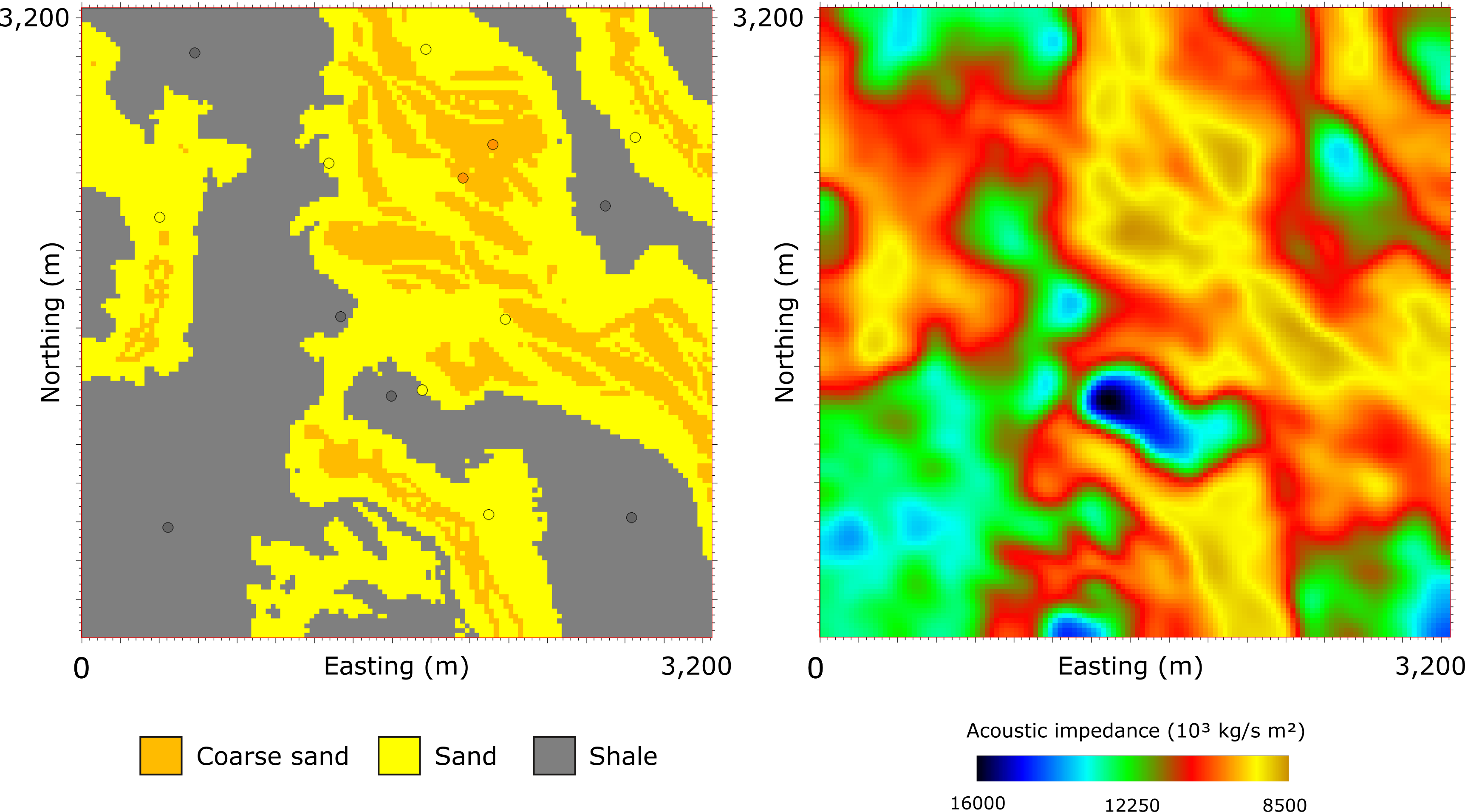
The fifteen conditioning data do not yield reliable indicator variograms. Thus, the experimental variograms are based on the geological reference image. The variogram model for all facies is exponential, anisotropic in the direction of 120°, with major and minor ranges specified in the table below. The variograms have no nugget effect. Indicator variograms should have no nugget effect unless the discretization of the data is very coarse with respect to the size of the categorical units.

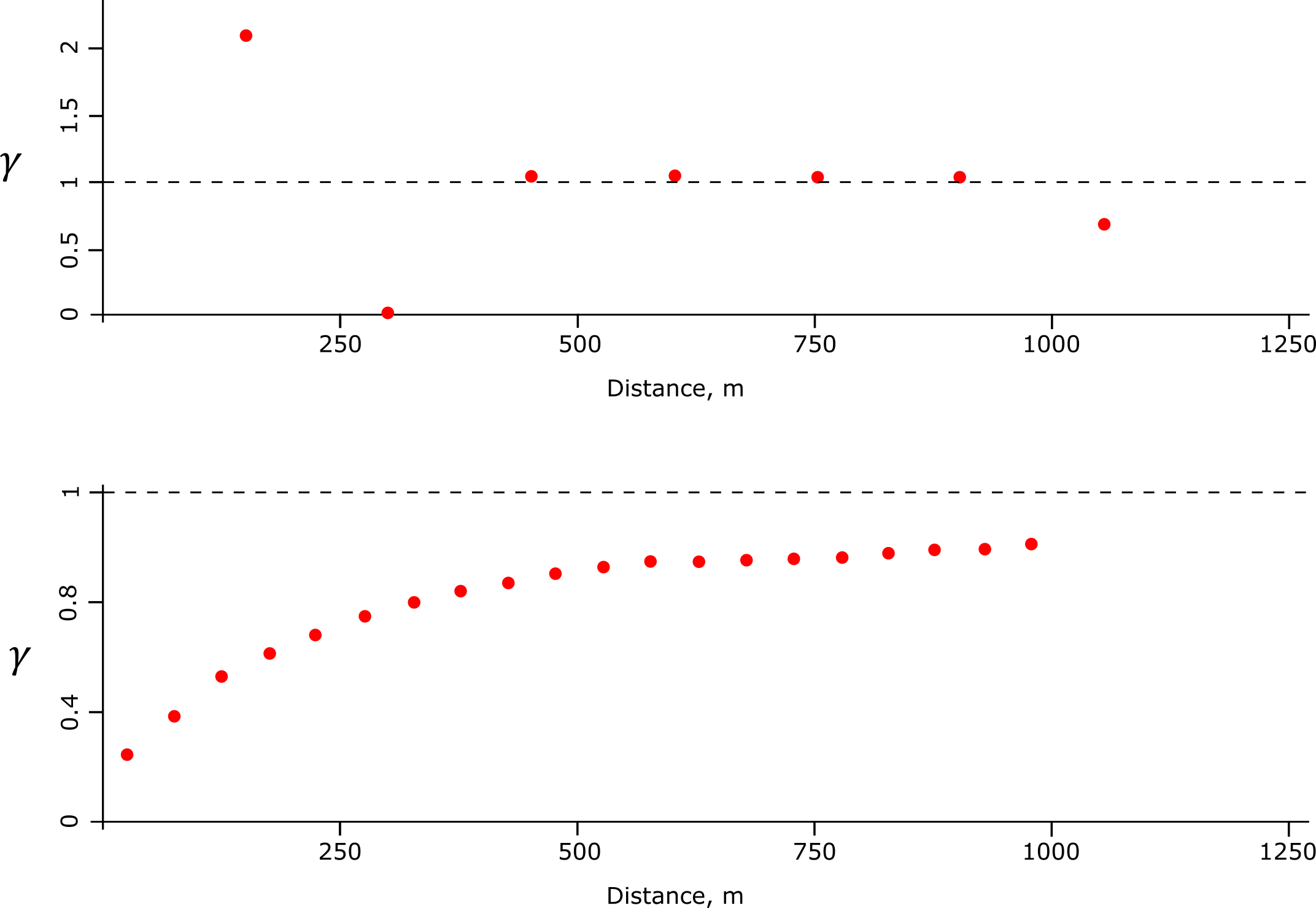
Sparse data could lead to misinterpretation of the variogram (Pyrcz & Deutsch, 2014) including a too high nugget effect. Detailed data are usually not available to obtain stable horizontal variograms. The horizontal variogram could be inferred from a horizontal/vertical anisotropy ratio from conceptual geological models (Kupfersberger & Deutsch, 1999). Commonly, the vertical variogram is stable due to the dense sampling along vertical wells. Seismic is another option to infer the horizontal variogram ranges. In all cases it is crucial to define the variogram considering a site specific local geological conceptual model. The experience of the modeler is significant to variogram modeling. Variograms selected for this environment have major/minor ranges of 700/400 for coarse sand, 500/350 for sand, and 900/650 for shale.

For simple kriging in this example, the global mean values come from the reference image: 13% coarse sand, 39% medium sand, and 48% shale. The locally varying mean was constructed from the synthetic acoustic impedance and the geological reference image through a direct transformation using linear functions from the acoustic impedance distribution for facies. These linear functions can be considered as conditional expectations of the facies proportions given acoustic impedance.

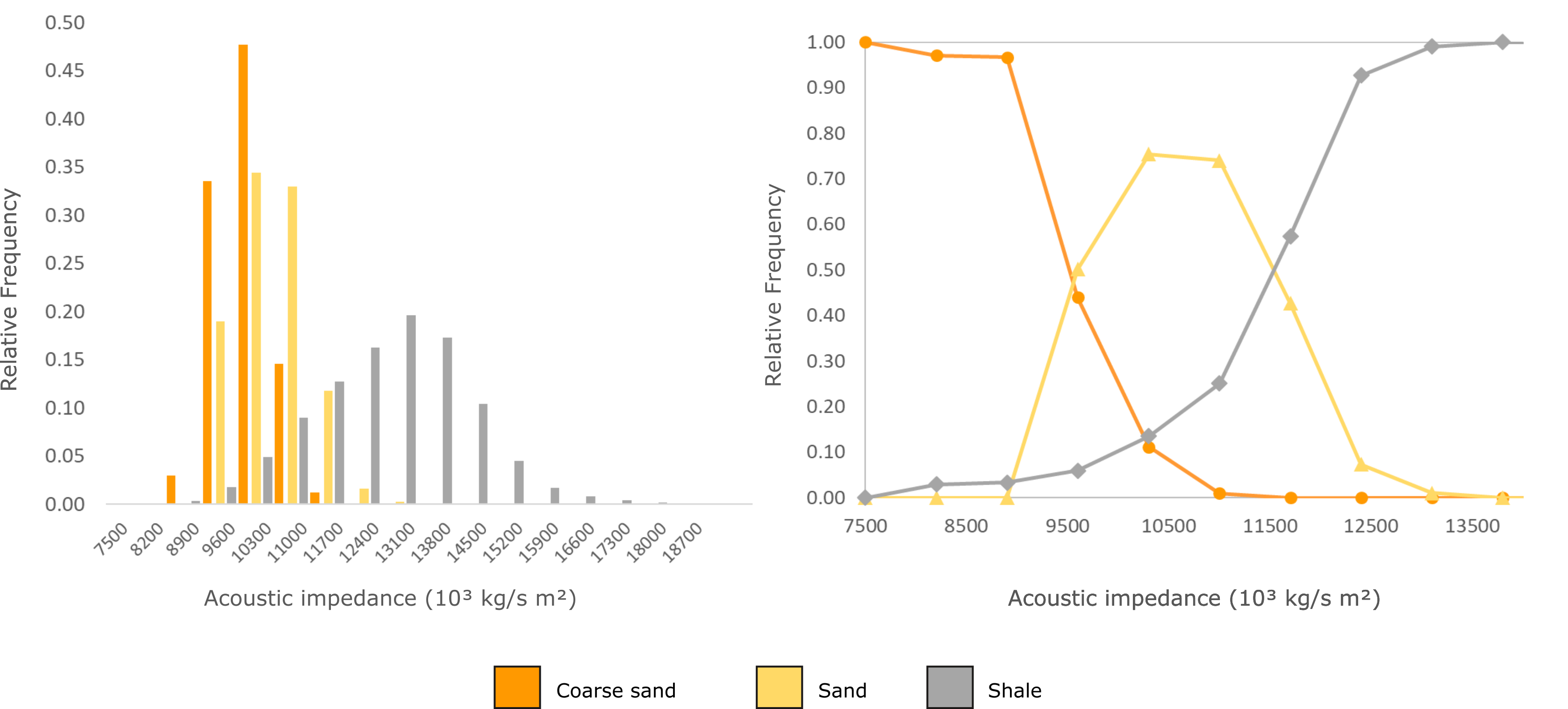
This procedure requires a significant amount of data to be representative of the distributions. An alternative is to consider Bayes theorem applied to the secondary data (see lesson: An Application of Bayes Theorem to Geostatistical Mapping).

Two hundred realizations from each method were simulated using the same data and variograms.

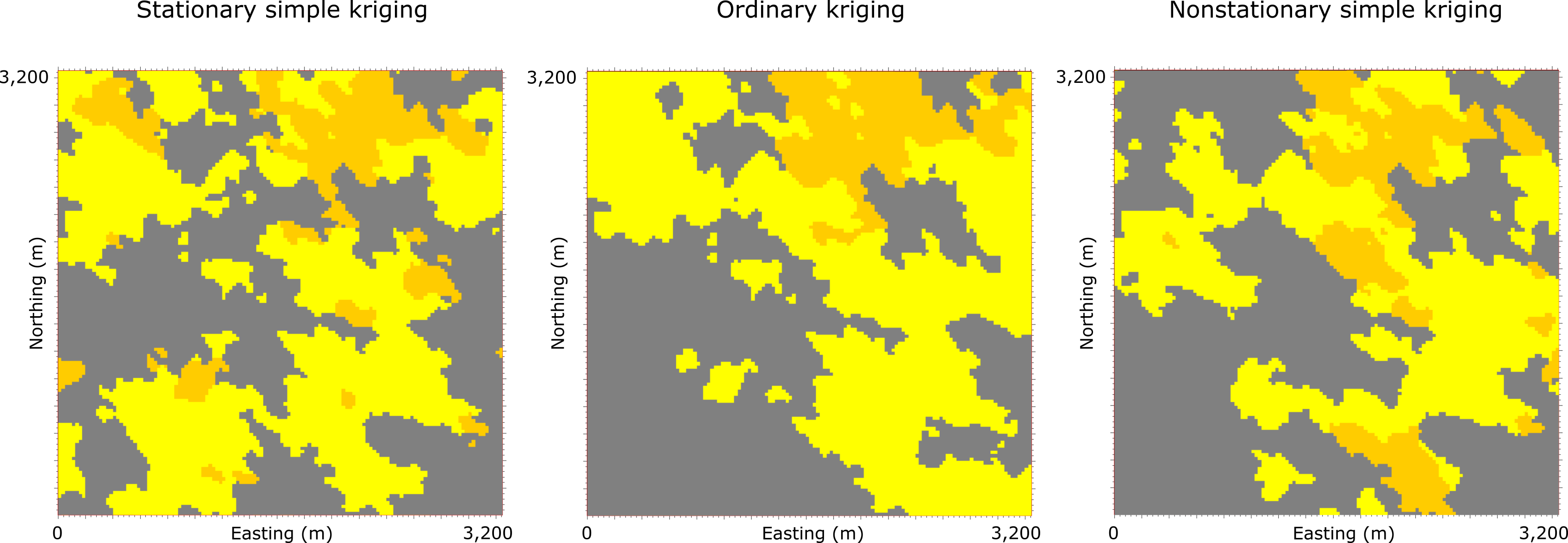
Accuracy and entropy allow an evaluation of the realizations. Accuracy compares the realizations and the reference image. It is defined here as the proportion of times the nodes are correct. The SK method presents the lowest accuracy, 0.46, followed by the OK, 0.50, and the highest for LVM is 0.59. Journel and Deutsch (1993) (A. G. Journel & Deutsch, 1993) describe entropy in geostatistics as a measurement of the uncertainty for a distribution model.

\[ H = - \sum_{k = 1}^{K} [\ln p_k]p_k \geq 0 \]

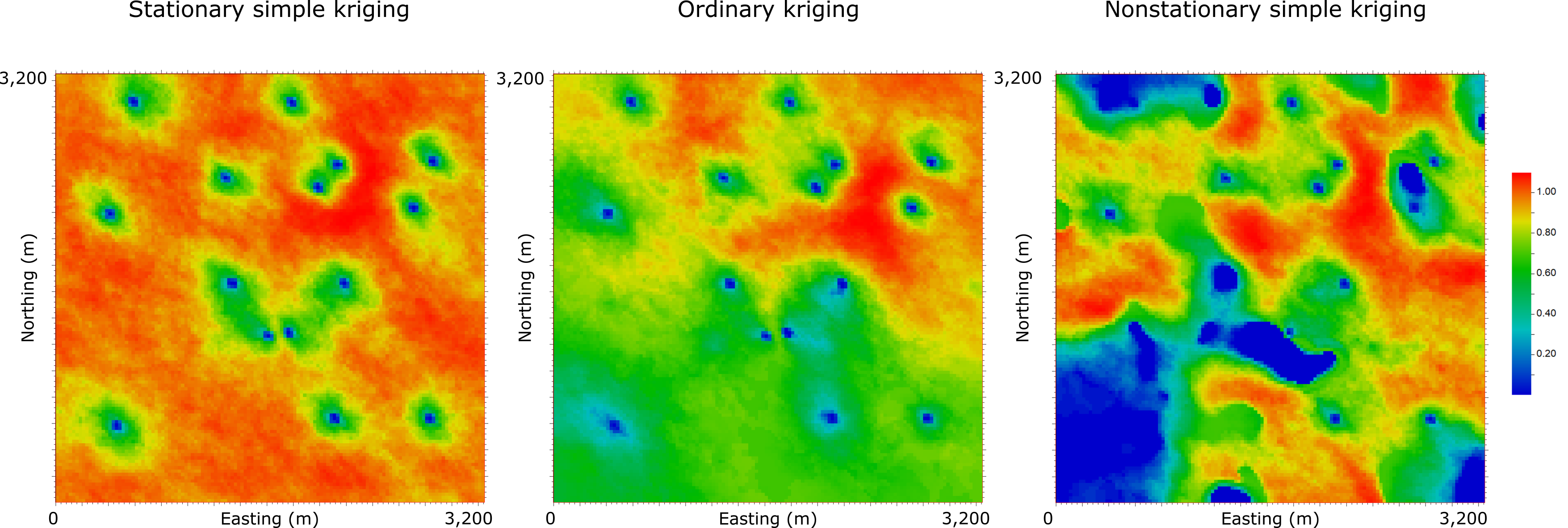
The entropy maps for each method are shown. The entropy maps highlight differences in the methods. The SK entropy is the highest, with an average of 0.98. The high values are homogeneously spread away from the data, reflecting the variogram and dependence on the global average. The OK entropy, on the other hand, has a lower average entropy of 0.75. Regions between samples of the same facies have lower entropy, see the southwest. Areas with three different facies have higher entropy, see the northeast. The LVM has the lowest average entropy of 0.67. There are regions with entropy close to zero, even in areas beyond the variogram range. The local mean or proportion maps from seismic control this behavior. For instance, where high impedance values occur, above 12500(10³ kg/s m²), the probability of shale approaches 1, decreasing the uncertainty. There are areas where the LVM maps increase uncertainty, but on average, the secondary data reduces uncertainty and increases accuracy.

Discussion

SIS has received several criticisms. Emery (2004) (Emery, 2004) mentioned problems related to the indicator formalism: difficulties in honoring the model parameters and indicator correlograms leading to problems in multipoint statistics. Another common criticism is the limited capacity to reproduce the complexity of some geological bodies, especially curvilinear (Caers & Zhang, 2004; Strebelle, 2002), caused by the limitation of two-point variogram statistics. In addition, the already mentioned excessive variability, not consistent with some geological features (Deutsch, 2006). There are three main alternatives for facies modeling: Truncated Gaussian Simulation (TGS), Object modeling, and Multi-point statistics (MPS).

TGS is also a variogram-based technique presenting similar results as SIS (Galli, Beucher, Le Loc’h, Doligez, et al., 1994). Some differentiating features include greater control on facies transitions, non-constant proportions defined by vertical proportion curves, horizontal constraints, and images smoother than SIS, resulting from the Gaussian model. It is suitable for a geological environment with low variability and well-defined facies transitions.

Object modeling is the stochastic simulation of objects described by a mathematical model. The expected geometries for respective facies determine the choice of the objects, usually defined by shape, direction, size, and frequency. A typical example of object modeling is fluvial channels (Deutsch & Wang, 1996; Holden, Hauge, Skare, & Skorstad, 1998), where curvature and continuity are better represented than using variogram-based algorithms. Zhou (2018) (Zhou, Shields, Tyson, & Esterle, 2018) discusses the low capacity of the SIS to reproduce fluvial channels relative to object modeling. The most significant object modeling restriction is the limited number of objects and challenges of conditioning.

Multi-point statistics (MPS) algorithms are another alternative. The parameters used to define the spatial continuity are established with multiple point statistics calculated from a training image. The advantage is to extract complex structures from geologically realistic images. Although training images are challenging to define, mainly because of stationarity requirements (Caers & Zhang, 2004), MPS has potential in certain circumstances.

No solution is appropriate for all geological contexts. For that reason, the selection of a facies modeling algorithm should consider spatial distribution characteristics of the modeled facies. SIS is a simple solution with straightforward parameterization when the facies distribution is easily described by anisotropic variograms, especially in settings with high variability and complex facies transitions. Considering the different options of SIS, the LVM is a reasonable option when secondary information is available.

References