Learning Objectives

• Appreciate high dimensional distance calculations with geological data
• Understand multidimensional scaling (MDS) within the framework of multivariate geostatistics (source code available).
• Interpret results from MDS to help understand multivariate data

Introduction

Multidimensional scaling (MDS) (Kruskal, 1964; Shepard, 1962; Torgerson, 1952) is a method used in data sciences to visualize and compare similarities & dissimilarities of high dimensional data. Its use in geostatistics helps visually assess and understand multivariate data in a lower dimension. By reducing the dimensionality of the data one can observe patterns, gradients, and clusters that may be helpful in exploratory data analysis. MDS does this by projecting the multivariate distances between entities to a best-fit configuration in lower dimensions that we can see.

This lesson will summarize the basic theory behind the technique including data preparation. Interpretation of the results for multiple examples will hint at various applications. A Jupyter Python notebook example is provided.

Theory

Multidimensional scaling is a family of algorithms aimed at best fitting a configuration of multivariate data in a lower dimensional space (Izenman, 2008). If the magnitude of the pairwise distances in original units are used, the algorithm is metric-MDS (mMDS), also known as Principal Coordinate Analysis. However, if magnitudes are unknown, it is possible for similarities from a higher dimension to be rank ordered and projected to a lower dimension which is known as non-metric MDS (nMDS). Dissimilarity and distance are interchangeably used to describe the difference between entities, whether a physical distance or some quantification of relatedness.

Suppose there are \(n\)-entities (eg. drillholes) and \(n(n-1)/2\) pairs with each pair having a measure of distance. The distance is a function of many variables for each entity (eg. mineralization, alteration, lithology, location, grade, length, year drilled). MDS takes the pairwise distances between the entities and finds best-fit representations of the points in all lower dimensional spaces. We commonly visualize the 2 or 3-D representation.

Data Preparation

The entities and variables are selected first. The variables are chosen to reflect the goals of the study. The data must have no missing values.

Variables are often standardized for consistent distance calculation. Consider \(n\)-entities, \(i=1,...,n\) and \(K\)-variables, \(k=1,..., K\). A simple standardization is achieved by: \[x_{k,i}=\frac{z_{k,i}-\mu_{k} }{\sigma_{k}}\] where \(z_{k,i}\) denotes the \(k\)-th variable of the \(i\)-th data in original units, \(x_{k,i}\) is the standardized data, \(\mu_{k}\) and \(\sigma_{k}^2\) are the mean and variance of the \(k= 1,...,K\) variables. Once standardized, each variable has a mean of zero and a standard deviation of one.

Distance matrix calculation

The distance between the different entities can be calculated by the Euclidean distance, correlation coefficients, or another method. The Euclidean distance is common:

\[d_{ij}=\sqrt{\sum_{k=1}^K(x_{k,i}-x_{k,j})^2} \:\: \text{for} \:\: i,j=\:1,...,n\]

where \(d_{ij}\) is the Euclidean distance between entity-\(i\) and entity-\(j\) for the \(K\) variables being considered.

Distances can also be calculated using correlation coefficients between variables. In this case, the variables are the entities (\(i,j\)) and the correlation coefficients (\(\rho_{ij}\)) between all variables form a similarity matrix. The distance or dissimilarity between the \(i\)-th and \(j\)-th entities (\(d_{ij}\)) is calculated by: \[d_{ij} = 1-\rho_{ij} \:\: \text{for} \:\: i,j=\:1,...,n\]

The distance matrix is essential for MDS.

Embedding

An optimization algorithm is used to embed the entities in a lower dimension space with pairwise distances as close as possible to the input distance matrix.

A simple example of 4-entities with 3-variables is shown below:

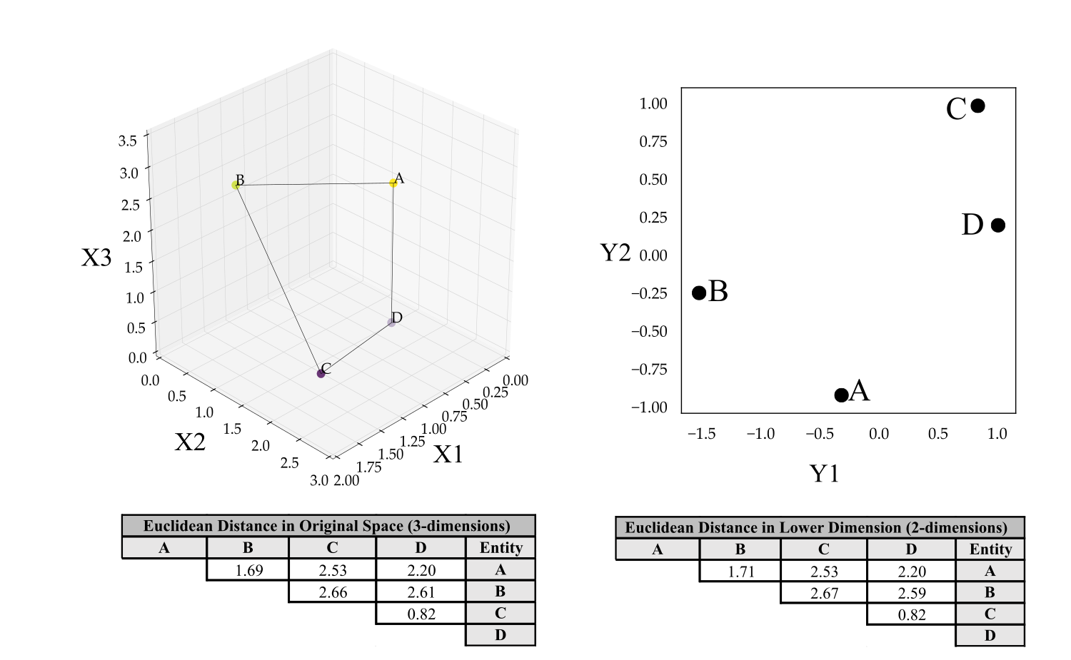
The distances between entities in the lower dimensions are not preserved exactly. MDS finds the best-fit configuration. The distortion in distances between the lower dimension and higher order space is called stress, which is minimized by the MDS implementation.

The axes (\(Y1, Y2\)) in lower dimensions are ordered from largest range of variability to least (Cox & Cox, 2001).

Examples

Northwest Territory Data

A set of data assembled by the Northwest Territories Geological Survey consists of n=8503 surface samples (Falck et al., 2012). The 36 elemental variables are chosen for exploratory data analysis. The correlation matrix is shown below.

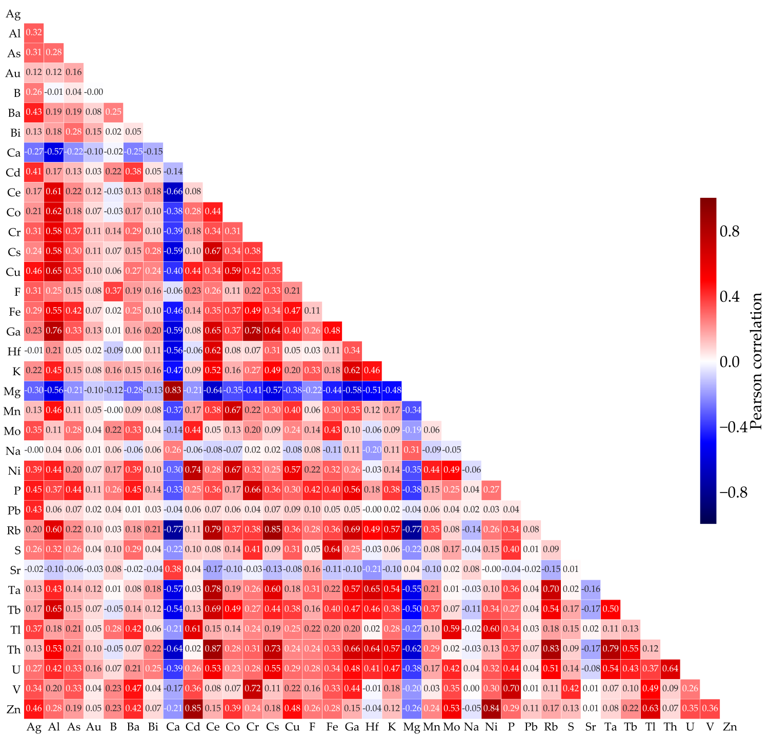
The 36 dimensional multivariate space of the variables cannot be visualized. The distances \(d_{ij}=1-\rho_{ij}\) are embedded using scikit-learn’s MDS implementation (Pedregosa et al., 2011) and shown below.

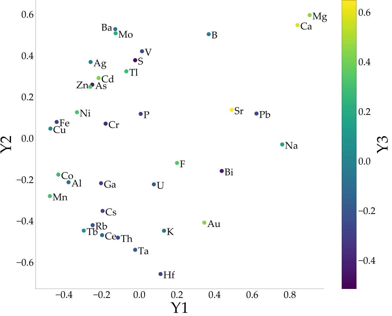
Some interpretations based on this plot include the following. Calcium (Ca) and Magnesium (Mg) appear together as outliers in the upper right of the plot. They are largely negatively correlated with the other elements from the correlation matrix with the exception of Strontium (Sr), which is also an alkaline earth metal and appears close in the MDS plot. The transition metals Mn, Co, Cu, Fe, Ni, Cr, Zn, Cd, Ag, V, Mo appear as a gradient on the left hand side of the plot, while Hf and Au, also transition metals, are distal to this gradient. The strongest correlation from the matrix is \(0.87\) between Cerium (Ce) and Thorium (Th). Lead (Pb) appears to be largely uncorrelated with all elements and thus plots far away on the \(Y3\) axis. The \(Y1\) axis shows the most variability while \(Y2\) is intermediary, and \(Y3\) exhibits the least.

Mining Economic Data

As another example consider economic, stock, and mine production data from company disclosures. These examples are strictly for educational purposes and should not be misconstrued as financial or professional advice. Medium sized gold producing companies (n=14) are compared in order to understand the relationship between different measures. There are 12 variables reduced to 3-dimensions using MDS. A correlation matrix of the variables was calculated and MDS used distances given by \(d_{ij}=1-\rho_{ij}\):

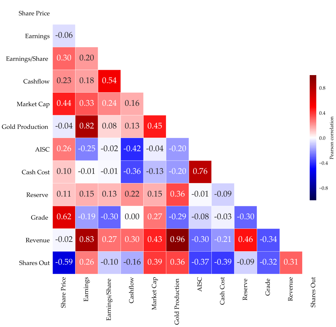
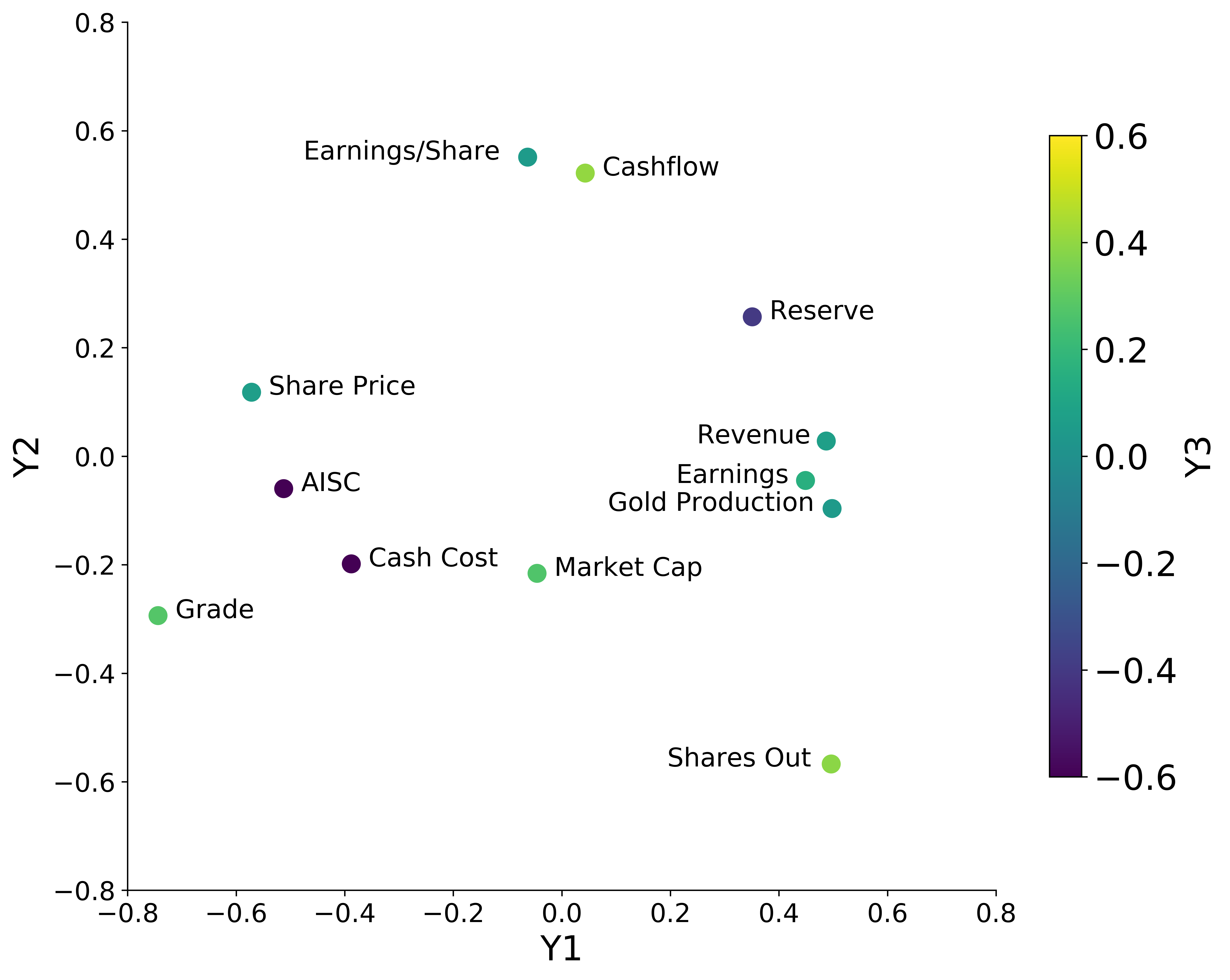
Distinct clusters and gradients can be observed. Between Gold production, Market Cap, Earnings, and Revenue, a gradient and cluster can be noted. Cash Cost per ounce, a measure of the operational cost to mine an ounce of gold, and All-In-Sustaining-Costs (AISC), reflecting the full cost, are closely related whilst Shares outstanding and Grade appear to be outliers.

Correlation based distance has been used in the two examples; however, Euclidean distance can be used to calculate distance. As an example consider the 14 medium sized gold producers as the entities with the aforementioned 12 variables. The distance matrix is generated by standardizing the 12-variables and calculating the Euclidean distance to be input directly to MDS.

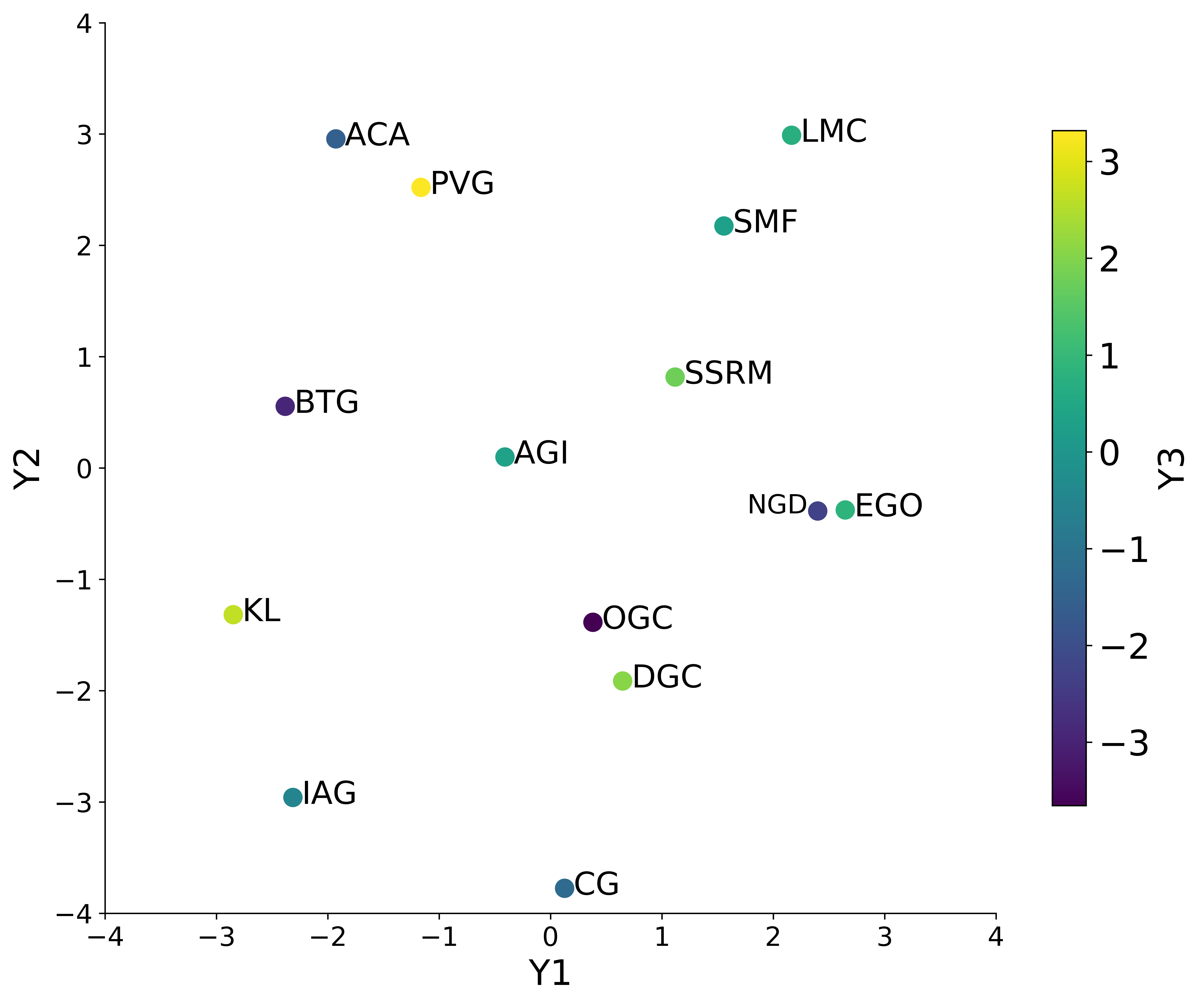
The companies are spread rather uniformly over the principle axes (\(Y1, Y2, Y3\)) with the exception of Kirkland Lake (KL) and to an extent Pretium Resources (PVG). Kirkland Lake is an outlier because of its high-grade (1.82\(\sigma\)), high ounce production (1.72\(\sigma\)), at relatively low cost (AISC=0.51 \(\sigma\)).

Some Other Applications

Geostatistical realizations represent possible outcomes of the uncertainty model (Barros & Deutsch, 2017). The realizations (n=100-200) are considered as an ensemble. Barros & Deutsch 2017 proposed the use of MDS to help optimally order realizations for visual analysis and presentation. An algorithm was developed to sequentially display realizations as a function of their inter-item distances.

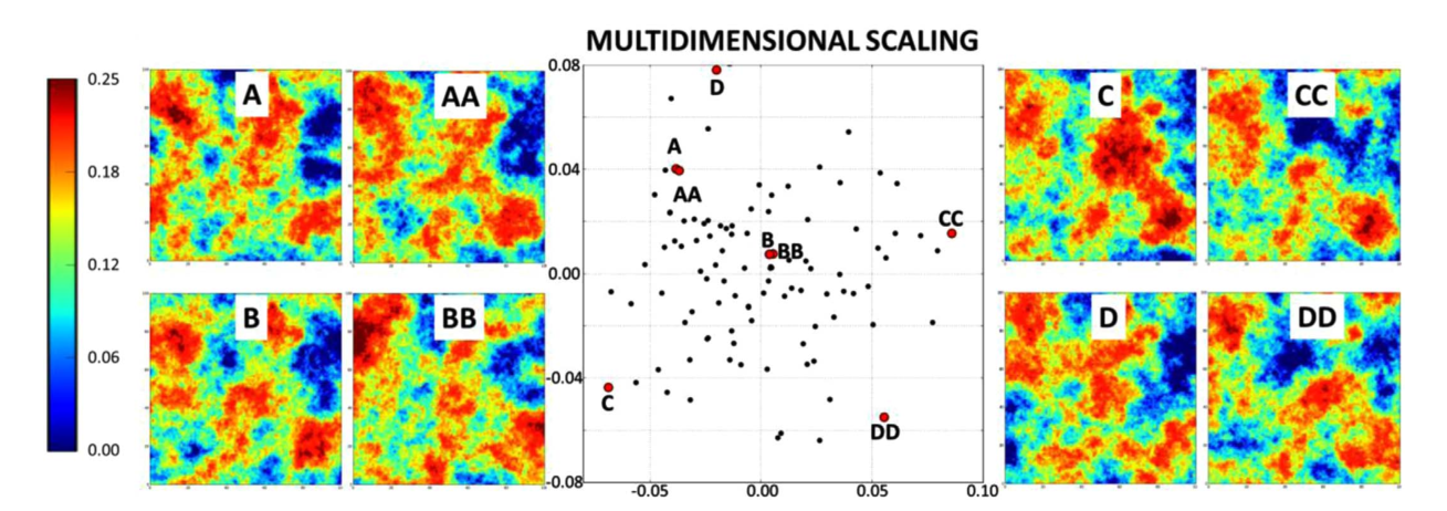
The distances are used to find shortest path route through the realizations. The result is a smooth optimal ordering of realizations to help the analyst better visualize and interpret the realizations and uncertainty. A video playlist of 2 case studies contained within Barros & Deutsch 2017 show the effect of optimal ordering in the visual assessment of uncertainty pertaining to simulated realizations.

Anisotropy in geostatistics outlines the directional dependence of the continuity of geological variables (Boisvert, 2010). Locally varying anisotropy (LVA) occurs naturally in geological systems. For example, folding and faulting of sedimentary beds can lead to a change in the principal directions of continuity. Considering LVA in the distance calculations may result in covariance matrices that are not positive definite. The LVA-based distances could be embedded in a Euclidean space that closely honors the distances in the original LVA-space and ensures positive definiteness in kriging calculations (Boisvert, 2010).

Modeling of geological variables is more complex and of a higher dimension than the target response. An output can be a simple binary response; however, there are many locations and multiple variables creating a high dimension. Embedding into a lower dimension metric space increases the efficacy and efficiency of interpretation and relating the response to geological characteristics (Caers, Park, & Scheidt, 2010). The connectivity distance between realizations could be considered.

Summary

Multidimensional scaling is a practical tool to help understand multivariate data. The embedding of high dimension entities in lower dimensions allows for convenient visualization and other calculations. We could identify clusters, outliers, and gradients. The assessment of these features provides a better understanding of the multivariate system.

References