Learning Objectives

• Understand the place of localization
• Review the steps to localize probabilistic resource models
• Compare localized simulation, localized uniform conditioning, and localized indicator kriging models

Introduction

Recoverable resources for both surface and underground mining at a chosen mining selectivity must be predicted from sparse exploration drill hole data. Grade control sampling at the time of mining provides orders of magnitude more data and much better estimates than possible with exploration data. Probabilistic methodologies anticipate this information effect with distributions of possible outcomes. Common probabilistic methods include simulation, uniform conditioning (UC), and multiple indicator kriging (MIK). These methods generate a distribution of possible grades at unsampled locations.

Managing the uncertainty represented by these models is a challenge. Many mine planning operations require a single deterministic model as input. Localization creates a single model from the distribution of possible values for the unsampled locations. Localization was initially proposed as an extension of Uniform Conditioning (Abzalov, 2006), but can be straightforwardly extended to multiple Indicator Kriging (Hardtke, Allen, & Douglas, 2011), MultiGaussian Kriging (Daniels & Deutsch, 2014), and Simulation (Boisvert & Deutsch, 2012) (with Sequential Gaussian Simulation, Turning Bands, and variants with trends as common options). This lesson provides an overview of the localization process and discusses the pros and cons of the approach.

An alternative to localization is to estimate a single resource model with ordinary kriging or inverse distance. The search or other estimation parameters would be restricted to calibrate the smoothing to a change of support model, detailed in the Lesson on choosing a kriging plan. Comparing a probabilistic model with a single resource model generated by estimation can be challenging. Localizing probabilistic results, however, generate to a single model consistent with the source probabilistic models.

Scales of Relevance

Regardless of the geostatistical method, there are four scales that are important to the localization process. The domain (\(A\)), the data scale, the selective mining unit (SMU) scale, and the panel scale, represented in the figure below. These scales are relevant for surface mining where there is significantly more data and some flexibility at the time of mining. The concept of a stationary domain (denoted \(A\)) is central to all geostatistical modeling. Localization proceeds within stationary domains. The domains should be relatively large to include 10s to 100s of panels. They should be geologically homogeneous with chosen stationarity, and the domain limits should be reasonably certain. Localization of probabilistic geologic models should consider the nature of the boundary when selecting a localization strategy (to localize across boundaries or not).

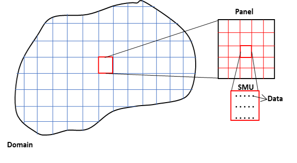
At the other end of the spectrum is the data scale. The composites used for resource modeling are the data scale. Although there may be many data, only a small portion of the deposit is actually sampled; often less than one billionth of the mass of a deposit is drilled. Experimental data for geostatistical analysis are rarely collected on a regular grid. A representative distribution for the domain must be inferred.

The selective mining unit (SMU) is a small regular block size that represents future mining practice considering mining equipment, available data at the time of mining, geological controls, mining operations including blasting and other aspects. A better informed ore control model will be used to determine the destination of mined material at the time of mining, but the SMU size anticipates future mining practices (Rossi & Deutsch, 2014). The SMU size is chosen as the block size that would lead to the same reserves as mined with the anticipated equipment, operational considerations, and grade control information availability. In an open pit setting, SMUs are typically the bench height and some multiple (1 to 3) of the grade control data spacing considering the mining equipment (Rossi & Deutsch, 2014).

In addition to determining a reasonable SMU size, the localization workflow requires the selection of an appropriate panel size. A panel is a group of SMUs. The SMUs need not be contiguous within the panels; however, that is the common choice. A panel is a large volume containing 10s to 100s of SMUs. The localization process considers that the distribution of SMUs within each panel is well-informed and adequately discretized. The localized model is not considered reliable at smaller scales. Thus, the panels should be large enough to provide a reliable SMU distribution within the panel and small enough to provide local precision. There is no evident optimal panel size, but panels that are one to two times the bench height and with a total of 50 to 100 SMUs within the panel are considered reasonable. The geometry of the panels should be carefully considered. The panels should be close to large volumes that could be mined in the future. The panels should also be as homogeneous as possible, for example, if the mineralization has a strong vertical continuity, then the panels should have a significant vertical extent.

SMU Scale Distributions of Uncertainty

Uniform conditioning (UC) directly predicts the SMU distribution within a panel. Simulation is most often at the point scale; simulated realizations are block averaged to the chosen SMU scale to directly provide the SMU distribution at each location. MutiGaussian Kriging (MGK) and multiple Indicator Kriging (MIK) predict uncertainty at the point scale; therefore, a change of support model is applied to convert the results to the appropriate SMU size. Multiple methods have been developed for change of support. The affine correction and indirect lognormal correction are simple methods that provide approximate results. The Discrete Gaussian Model (DGM) considers a fit to the point scale distribution and an analytical change of support that is quite flexible. Considering a global correction to each local distribution inferred by MGK or MIK is an assumption given that the local corrections would depart from the global correction. The common options for SMU uncertainty are now described.

Simulation

Simulation is often preferred because it allows the generation of realizations that reproduce the variability of the underlying random function, and can manage non-stationarity within a domain using a trend model. Multiple realizations represent uncertainty about the spatial distribution of the grades. There are many simulation algorithms, and they are often nested, that is, rock types may be simulated first, then continuous grade values. The sequential Gaussian simulation (SGS) algorithm is widely used. SGS makes the same assumptions as multiGuassian Kriging but quantifies uncertainty through a set of realizations rather than local conditional distributions. For each location in a realization a simulated value is drawn from the local conditional distribution and then retained to condition subsequent locations. Considering previously simulated values preserves joint uncertainty between all locations. Simulation takes place at the data scale and reproduces the histogram and variogram of the variable being modeled. A set of realizations are generated at the data scale and averaging to blocks is applied to represent the SMU scale uncertainty.

Sequential Gaussian Simulation requires all variables to be transformed to a standard normal (Gaussian) distribution. The conditional distribution for a variable at an unsampled location is calculated in Gaussian units. The normal equations are utilized to compute the local mean and variance that define the local distribution. The conditioning includes all original data and previously simulated values available within a neighborhood. A value is drawn randomly from this distribution and retained as the simulated realization at this location. This simulated value is also incorporated into the set of data available for conditioning future distributions. This process is repeated for the entire grid, retaining a simulated value at each location to complete a realization. The simulated values are averaged within each SMU volume to generate a set of SMU scale realizations. These distributions of SMU grades are an input to localization.

Uniform Conditioning

This technique estimates the tonnage and grade at an SMU scale that could be extracted from larger panels. The key steps in the UC procedure include (1) fitting the data scale distribution by a series of Hermite polynomials, (2) inferring the SMU scale and panel scale distributions using the data scale distribution and the volume averaged variogram values within the SMU scale and panel scale, (3) ordinary kriging at the panel scale, (4) transforming the panel scale estimates to Gaussian units, (5) extract the distribution of Gaussian SMU values from the bivariate distribution of Gaussian panel and Gaussian SMU values, and (6) back transform the Gaussian SMU distribution at each location to original grade units. The key assumption of UC is that the bivariate distribution of Gaussian panel and Gaussian SMU values is bivariate Gaussian defined by a stationary correlation coefficient. This assumption requires stationarity and uniform conditioning. The ore tonnage at the SMU scale and the grade of the recoverable tonnage is calculated from the local distributions without exactly specifying the position of the ore grade SMU blocks. To arrive at one SMU grade per SMU location, Localized Uniform Conditioning (LUC) was proposed by Abzalov (2006) as a way to spatially locate the SMU grades determined by the UC technique. The SMU distributions within each panel are a direct input to localization.

Multiple Indicator Kriging

Simulation and UC depend heavily on the multivariate spatial Gaussian distribution. Multiple Indicator Kriging is non-parametric where the distribution is estimated via binary indicators (Journel, 1983). Multiple indicators are kriged and local distributions are constructed through post-processing to generate conditional distributions at the SMU scale. To achieve this, MIK considers a series of threshold values chosen from the representative global distribution. Often between 7 and 15 thresholds values are chosen. A variogram model is required for the indicator values (1 if below and 0 if above) at each threshold. The cumulative distribution function (CDF) is estimated at each threshold at each unsampled location (Deutsch & Journel, 1998). Order relation corrections may be required to ensure that each series of indicator estimates is non-decreasing within the range of 0 to 1.

The MIK-derived distributions represent a probabilistic model for the uncertainty in the composite-scale grade at unsampled location (Deutsch & Journel, 1998). These MIK-derived distributions must be post processed to represent the SMU scale. First, the resolution between thresholds is increased by interpolation or considering the shape of the global distribution. There is no theory developed for the correct local change of support, but it is common to apply a global change of support correction to the local distributions (Hardtke et al., 2011).

Methodology

The first step in localization is to assemble a distribution of SMU grades within each panel. Local SMU distributions within the panel are combined to form a single distribution for each panel, see Figure below for a schematic illustration. As mentioned, panels are often defined as a rectangular volume containing 50 to 100 SMUs. The panel size does not depend on details of the mining operation, the mine plan, size of equipment or other considerations. The SMUs should nest neatly within the chosen panel grid. Ultimately, the goal of localization is to have one SMU grade for each SMU grid location.

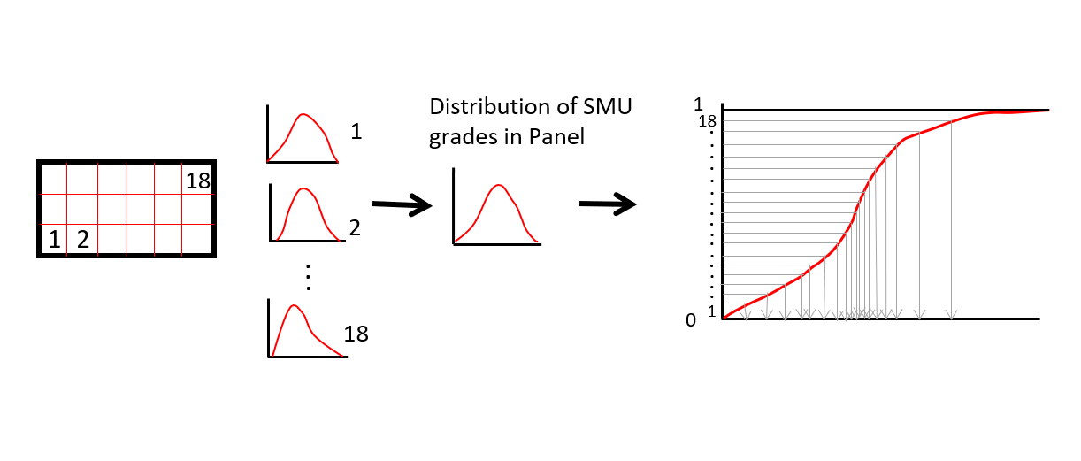
The second step is to discretize the combined distribution of SMU grades for each panel. The aim is to extract the exact number of grades from the distribution as there are in the panel. The number of SMUs in each panel can vary because of intersecting geological boundaries. In any case, the exact same number of discretization classes are considered as there are SMUs within a panel. Each grade class is of equal probability. The mean values, median values or randomly drawn values are kept from each grade class. Using the mean is simple and unbiased. The result of this step is a set of SMU grades for each panel - the exact number required for each panel.

The third and final step is to assign each of the chosen SMU grades to an SMU in the panel. Each panel is processed one at a time. It would be a bad idea to assign the SMU grades to random SMUs in the panel, the result would be very noisy. It would be a bad idea to assign the SMU grades in a regular order starting from the bottom left corner, the result would look very odd with artifact stripes. The central idea of localization is to place the low values in lower grade areas of the panel and the high values in high grade areas of the panel. A ranking or localizing variable achieves this purpose. Commonly, ordinary kriging at the SMU block scale is used to determine the ranking (Hardtke et al., 2011), or for simulation the e-type model used. This necessitates performing a very smooth kriging run separately from the determination of SMU uncertainty. The final model does not directly include the kriged grades, therefore avoiding any histogram smoothing. The lowest SMU value determined in step two is placed in the lowest grade SMU from the localized kriged grade in the panel. The value from the second grade class is assigned to the SMU ranked second according to the kriged grade. This is repeated until each SMU has a grade. The result is a single localized model considered representative of the SMU distributions within each panel (Boisvert & Deutsch, 2012). An example is shown below.

Example

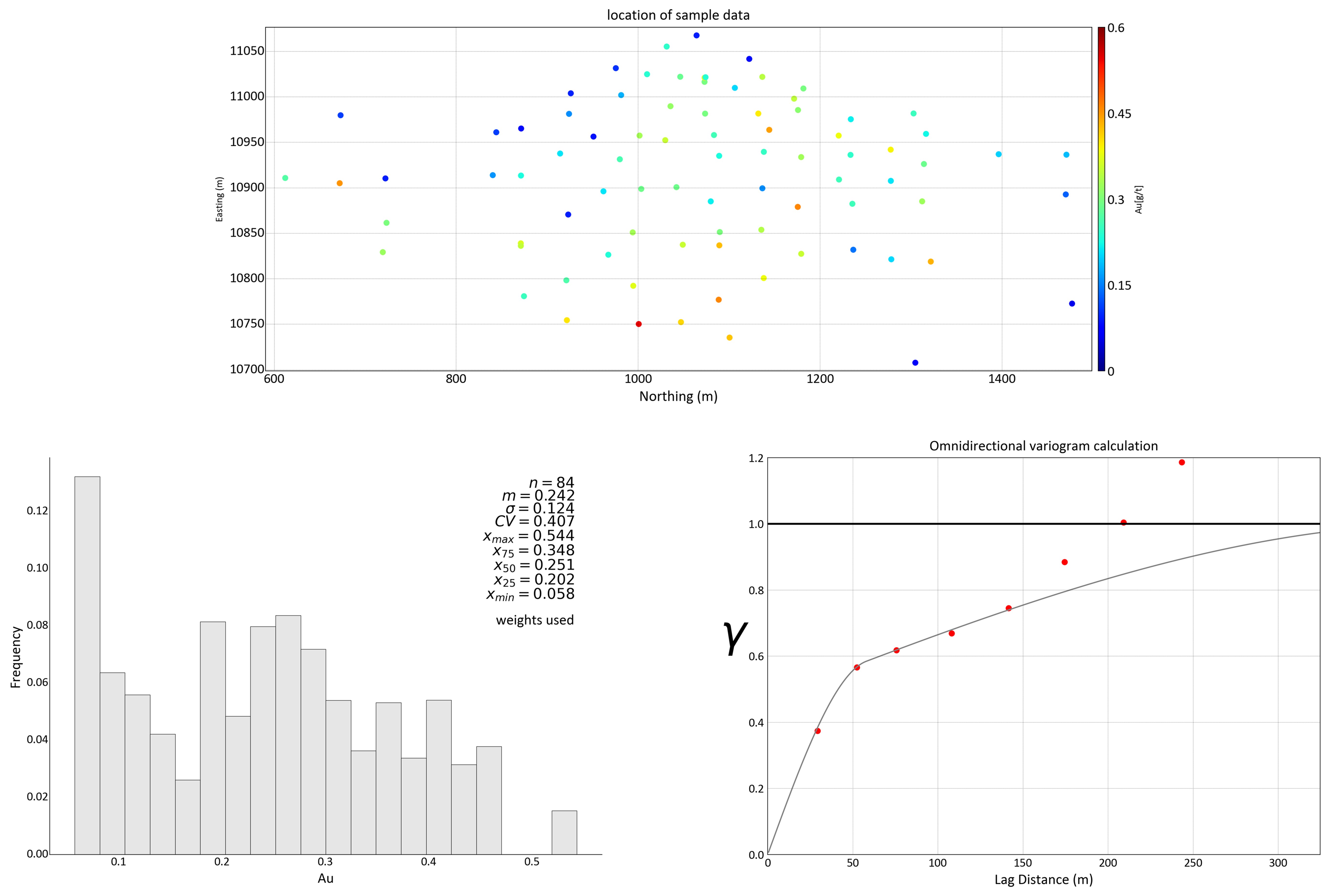
This example demonstrates localizing SGS, UC and MIK. This tabular deposit will be modeled in the two-dimensional plane of the structure. The dataset consists of eighty-four drill holes arranged irregularly across a 950m by 450m domain size. The grade distribution is positively skewed with a declustered mean of 0.242 and a variance of 0.0154, see below.

Cell declustering is performed with a maximum cell size of 150m. The data are transformed to normal scores for simulation; the variogram of normal scores is calculated and modeled for simulation. An omnidirectional isotropic variogram is considered, see figure below. One hundred data-scale realizations are simulated with sequential Gaussian simulation on a 1m by 1m grid. The realizations pass all the standard checks (see Lesson). The simulated realizations are back transformed into original grade units and block averaged to the SMU scale of 10m by 10m. The expected reduction in variance is accounted for in the block averaging.

Uniform Conditioning is applied with the steps summarized above. The result is a distribution of SMUs for each panel. In this simple example, there are the same number of SMUs in all panels, but this is not always the case in practice due to geological boundaries.

Nine thresholds were selected for MIK using the declustered histogram to resolve the predicted distribution and to avoid excessive order relations problems (Vincent & Deutsch, 2019). The threshold values are (0.095, 0.217, 0.243, 0.261, 0.319, 0.350, 0.386, 0.409, 0.444) corresponding to declustered CDF values of (0.1, 0.3, 0.4, 0.5, 0.65, 0.75, 0.85, 0.9, 0.95). Variograms are calculated and modeled for the indicator data at each threshold. Since the variograms relate to the same underlying continuous random variable, the transitions between the indicator variograms should be smooth in terms of variogram behavior (Vincent & Deutsch, 2019). Estimation parameters such as the number of data and search radius are chosen consistently with simulation. Ordinary kriging is generally used to estimate the probability distributions in indicator kriging because it is more resilient to non-stationarity. For post-processing, after order relations are corrected, construction of the complete posterior CDF occurs by interpolating between the estimated probabilities (at each threshold) and extrapolating into the tails. The minimum and maximum values are taken from the data.

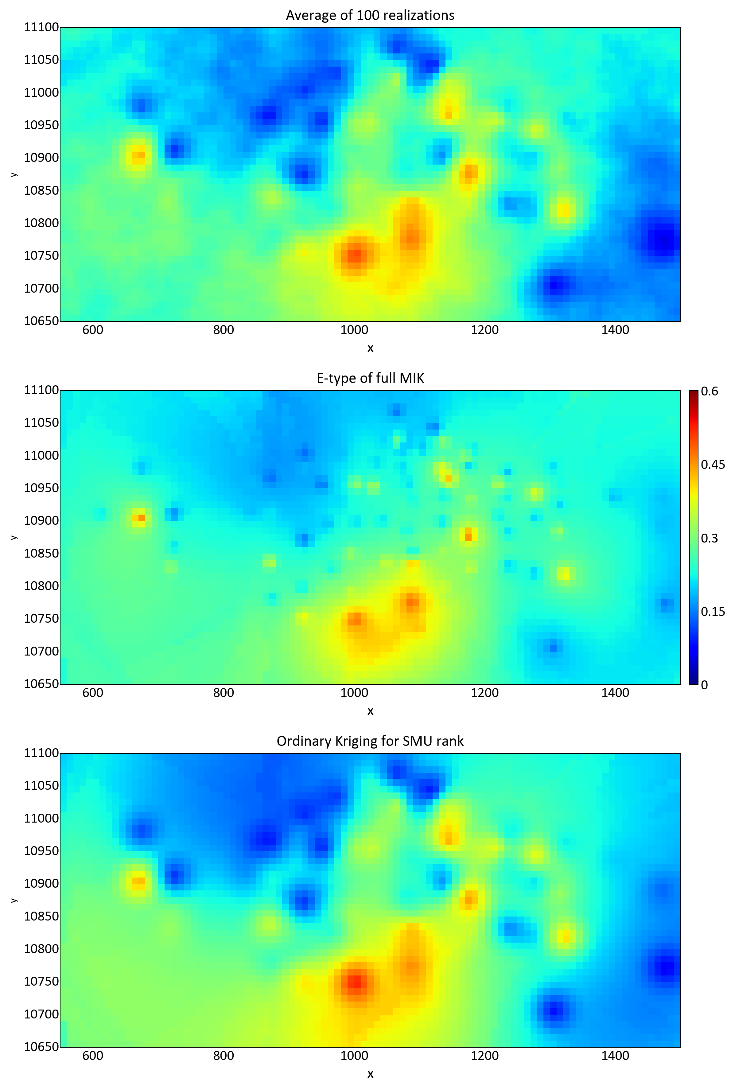
Each local distribution from MIK is corrected to represent the SMU support. A global change of support is considered with a global \(f\) value of 0.732 estimated from an average variogram value of 0.268. This uses the variogram in original units (not an indicator variogram), and that it is standardized, so the calculation is 1-0.268 to get the global \(f\). The SGS and MIK E-type estimates and the OK estimates are visually compared to the input data in plan view.

Localization

As preparation for localizing, a set of realizations have been simulated and block averaged to an SMU scale. In the case of UC and MIK, post-processing will generate a number of quantiles for localizing. Before the localization process, a localizing variable is required for ranking each SMU within the panels to assign the grades at the SMU scale. Standard practice is to generate an Ordinary Kriging model using the SMU grid definition. The workflow for localization of probabilistic models presented in this lesson requires 3 inputs:

• A gridded localizing variable at the SMU scale. This variable will be used to determine the rank of each SMU within a panel. Assigning grades from the SGS/UC/MIK model to the SMU blocks is based on a ranking of the SMU within each panel in increasing order of their grade. For this demonstration, ordinary kriging model is used as the localizing variable.
• An SMU scale model with a full distribution of uncertainty for each SMU. This is generated by post-processing the results from simulation, uniform conditioning and multiple indicator kriging.
• The panel definition assigns each SMU to an appropriate panel.

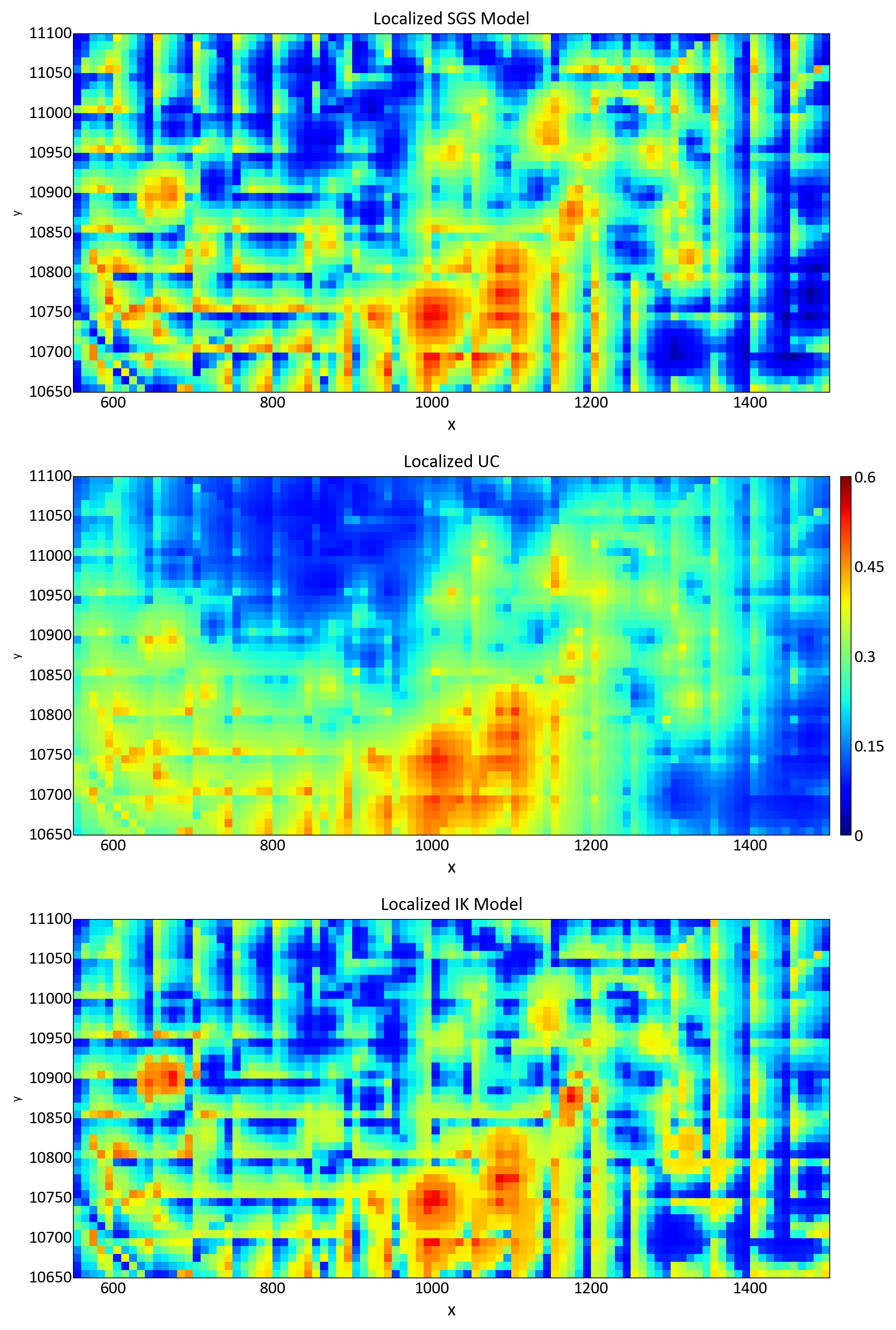
For the panel scale defined at a size of 50x50 and the SMU scale defined as 10x10, this results in twenty-five SMUs within each panel. These distributions are discretized into a series of twenty-five grade classes. The SMU scale localizing variable is used to rank each SMU within a given panel. The lowest value localized grade is assigned to the SMU of the lowest rank (lowest kriged grade) in the panel, the second to the second and so on until all SMUs receive a grade. The resulting distribution of the localized model is representative of the SMU distributions (Boisvert & Deutsch, 2012).

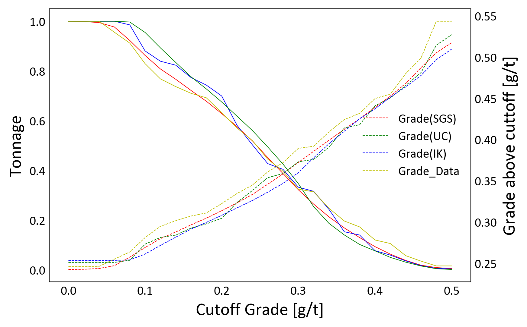
The results from localizing the model of uncertainty generated by SGS, UC and MIK are shown below. The grade tonnage curves for the localized models are also shown. The block distributions from simulation, UC and MIK are smoother than the data distribution. The block distributions are not the same given the different assumptions that go into the different techniques.

Discussion

The purpose of localization is to create a single model that reproduces uncertainty at the panel scale. This facilitates the use of most mine planning software that allows the input of only one block model.

A concern of localization is visual artifacts in regions of transition from high to low grade. High and low values are located at the panel edges with high values in one panel juxtaposed with low values in another. Some work has been performed to reduce these artifacts; however, the localized model is only valid at the panel scale and the artifacts serve as a reminder of how much we should trust the model. If possible, conventional mine planning with a localized model should be restricted to the panel scale which could work long range planning. Maintaining and using a model of uncertainty is recommended.

The panel scale serves an important purpose in localization as a middle ground between the model of uncertainty and an estimated single model; however, there is no requirement that panels must be defined as a regular rectangular shape of contiguous SMUs. By randomly assigning each SMU to a panel there are no distinct panel edges to generate the edge artifacts. Also, Boisvert and Deutsch (2012) suggest that instead of using the centers of the grade classes, adding an element of randomness to the grade values chosen from each grade class captures the high and low extents of the CDF more accurately.

Localization provides an effective methodology for reducing a probabilistic model of uncertainty to one model for situations that may value histogram reproduction over local precision. Localized conditional simulation with a trend is a flexible methodology for matching an expected grade-tonnage distribution and simultaneously working with geostatistical realizations and a single model to facilitate mine planning.

References