Learning Objectives

• Understand the optimality of kriging estimates and the calculated weights
• Recognize counterintuitive results and their origins
• Identify practical situations where counterintuitive results require mitigation

Introduction

Most resource models in the mining industry are constructed by kriging. Each block estimate in the model is a locally linear estimate based on the nearby data; the weights are different for every grid block. The response surface created by the block model of kriged estimates is highly non-linear, reproduces the available sample data and considers a site-specific measure of spatial continuity. Kriging is the mathematically optimal solution for assigning weights to data when estimating at an unsampled location. Optimality is defined as minimizing the squared difference between the estimate and the unknown truth (Leuangthong, Khan, & Deutsch, 2011). The utility of kriging has been established by thousands of models and validation studies over decades. Notwithstanding the proven nature of kriging, there are implementation measures needed in practice to address concerns regarding the string effect and negative weights. These concerns arise due to redundant data.

Kriging

A fundamental aspect of geostatistics involves estimating a variable throughout a domain using the available data. It is essential to define reasonable stationary domains and determine their statistical parameters such as the mean, variance, and variogram model (Chilès & Delfiner, 2009). A well-established paradigm is to estimate the variable for each grid block with a weighted linear estimate (Leuangthong et al., 2011). Calculating the appropriate weights for the nearby data is crucial. Historically, geologic modelers assigned weights inversely proportional to the distance between the data and the grid block being estimated. However, this method does not account for site specific spatial continuity, consider complex data configurations or satisfy a clear measure of optimality (Leuangthong et al., 2011). Daniel G. Krige pioneered the work of optimal interpolation in spatial concepts using linear regression throughout the 1950s. In 1963, Georges Matheron formalized the techniques and coined the term “kriging”, in honour of Daniel G. Krige, to describe a technique for determining optimal weights in spatial estimation(Leuangthong et al., 2011). These weights minimize the estimation variance considering spatial correlation with the variogram.

Counter Intuitive Results

This lesson focuses on two scenarios where the kriging weights appear counterintuitive. These scenarios are the “String Effect” and “Negative Weights.” The String Effect occurs when large weights are assigned to the endpoints on a string of collinear data (see Fig 1). Negative Weights may occur even though the data value is positively correlated with the grid block location, commonly seen when a data point lies behind or is screened by other data (see Fig 2). (Deutsch, 1993) argued the large weights assigned to the endpoints of string data are inappropriate and offered practical solutions. This lesson aims to better understand these counterintuitive results, demonstrate they are mathematically correct, and show practical circumstances where mitigating steps are recommended.

Practical Circumstances and Mitigation

Practical circumstances exist requiring the mitigation of the string effect and negative weights associated with screened data. In certain deposit types, high grades often occur at geological boundaries. In this case, the string effect can lead to a positive estimation bias toward the center of the domain. Negative weights can create a halo of negative grade estimates around a high-grade data point (Deutsch, 1996). This happens because the high-grade point receives a negative weight when screened by other data points. If the grade is sufficiently high, the negative weight can overpower the positive weights assigned to the surrounding relatively low grade data, resulting in a negative grade estimate. These unwanted consequences are mitigated through search restrictions when kriging.

Theory of Kriging

Kriging is an estimation technique that employs linear weighting of data; nearby data points are typically assigned larger weights in estimation. The kriging weights are calculated by minimizing the error variance (Leuangthong et al., 2011). Consider an unsampled location \(\boldsymbol{(u_\square)}\) and \(\boldsymbol{(n)}\) nearby points \(\boldsymbol{(u_\alpha), \alpha=1, \ldots ,n}\). The estimate at the unsampled location \(\boldsymbol{Z^*_\square}\) is written as:

\[ \boldsymbol{ Z^*_{\square} - m = \sum_{\alpha=1}^{n} \lambda_{\alpha,\square} [z(u_\alpha) – m]} \]

Letting \(\boldsymbol{Y(u) = Z(u) – m}\) we can rewrite the equation as:

\[ \boldsymbol{ Y^*_{\square} = \sum_{\alpha =1}^{n} \lambda_\alpha y(u_\alpha)} \]

The assumption of stationarity implies the mean is 0, the variance is the same throughout the domain, and the expected values of a product of \(Y\) values, the covariance, is given by the modeled variogram.

\[ \boldsymbol{ E\{Y(u)\} = 0 } \]

\[ \boldsymbol{ E\{Y(u)^2\} = \sigma^2 } \]

\[ \boldsymbol{ E\{Y(u)Y(u')\} = C(u, u') = \sigma^2 - \gamma(u, u') } \]

The best estimate minimizes the error variance in expected value:

\[ \boldsymbol{ \sigma_{\epsilon}^2 = E\left\{\left(Y^*_{\square} - Y_\square\right)^2\right\} } \]

expanding the terms leads to:

\[ \boldsymbol{ \sigma_{\epsilon}^2 = E\left\{Y^{*2}_{\square} - 2Y^*_{\square} Y_\square + Y_{\square}^2\right\} } \]

the estimate \(\boldsymbol{\displaystyle\sum_{\alpha=1}^{n} \lambda_\alpha y(u_\alpha)}\) for \(\boldsymbol{Y^*_{\square}}\) is substituted into the equation leading to:

\[ \boldsymbol{ \sigma_{\epsilon}^2 = E\left\{\sum_{\alpha =1}^{n} \sum_{\beta =1}^{n} \lambda_\alpha \lambda_\beta Y_\alpha Y_\beta - 2\sum_{\alpha =1}^{n}\lambda_\alpha Y_\alpha Y_\square + Y_{\square}^2\right\} } \]

the expected value is brought into the equation:

\[ \boldsymbol{ \sigma_{\epsilon}^2 = \sum_{\alpha =1}^{n} \sum_{\beta =1}^{n} \lambda_\alpha \lambda_\beta E\{Y_\alpha Y_\beta\} - 2\sum_{\alpha =1}^{n} \lambda_\alpha E\{Y_\alpha Y_{\square}\} + E\{Y_{\square}^2\} } \]

the expected value of a product of \(Y\) values is the covariance \(\boldsymbol{C}\) (calculated from the modeled variogram):

\[ \boldsymbol{ \sigma_{\epsilon}^2 = \sum_{\alpha =1}^{n} \sum_{\beta =1}^{n} \lambda_\alpha \lambda_\beta C_{\alpha , \beta} - 2 \sum_{\alpha =1}^{n} \lambda_\alpha C_{\alpha , \square} + \sigma^2 } \]

This shows the error variance in terms of weights, \(\boldsymbol{\lambda}\), the variance, \(\boldsymbol{\sigma^2}\), the covariance between the data locations and the estimate location, \(\boldsymbol{C_{\alpha , \square}}\) and the covariance between all pairs of data, \(\boldsymbol{C_{\alpha , \beta}}\) (Rossi & Deutsch, 2013). Each term of the equation affects the estimation variance differently.

Term 3: \(\boldsymbol{\sigma^2}\) is the variance of the stationary population. If all data points are deemed irrelevant, all weights (\(\boldsymbol{\lambda}\)’s) are zero and the estimate defaults to the mean. The only non-zero component in the estimation variance equation is the variance. The error variance starts at the population variance and decreases as relevant data points are included.

Term 2: \(\boldsymbol{2 \displaystyle\sum_{\alpha =1}^{n} \lambda_\alpha C_{\alpha , \square}}\) represents the closeness of the data to the unsampled location. Closer data have a higher covariance, the negative sign in front of the term leads to a reduction in error variance as the covariance between a data and the unsampled location increases. The data value must also receive some weight for the error variance to reduce.

Term 1: \(\boldsymbol{\displaystyle\sum_{\alpha =1}^{n} \displaystyle\sum_{\beta =1}^{n} \lambda_\alpha \lambda_\beta C_{\alpha , \beta}}\) considers the data redundancy between all of the data points. High covariance between the data implies high redundancy which increases the error variance.

The kriging equations are derived by taking the derivative of the error variance with respect to each of the weights \(\boldsymbol{\lambda_\alpha}\) and setting them equal to zero for all \(\boldsymbol{\alpha = 1, \ldots, n}\).

\[ \boldsymbol{ \frac{\partial \sigma_{\epsilon}^2}{\partial \lambda_\alpha} = 0 - 2C_{\alpha, \square} + 2 \sum_{\beta =1}^{n} \lambda_\beta C_{\alpha , \beta} = 0 } \]

These are simplified to the following well known kriging equations:

\[ \boldsymbol{ \sum_{\beta =1}^{n} \lambda_\beta C_{\alpha , \beta} = C_{\alpha, \square} \quad \text{for} \quad \lambda = 1, \ldots, n } \]

Expressed in matrix form, the left-hand side matrix contains the data configuration. The right-hand side vector contains the relationship between each data point and the estimation location (Leuangthong et al., 2011).

\[ \boldsymbol{ \begin{bmatrix} C_{11} & C_{12} & \cdots & C_{1n} \\ C_{21} & C_{22} & \cdots & C_{2n} \\ \vdots & \vdots & \ddots & \vdots \\ C_{n1} & C_{n2} & \cdots & C_{nn} \end{bmatrix} \begin{bmatrix} \lambda_1 \\ \lambda_2 \\ \vdots \\ \lambda_n \end{bmatrix} = \begin{bmatrix} C_{1\square} \\ C_{2\square} \\ \vdots \\ C_{n\square} \end{bmatrix} } \]

These equations are well established in geostatistics and in other disciplines that require estimates from multiple data. The unconstrained solution is referred to as Simple Kriging (SK). It is common to constrain the sum of the weights to be 1 so that the mean is not used in the estimate; this is referred to as Ordinary Kriging (OK) (Rossi & Deutsch, 2013).

Note that (1) Kriging minimizes the error variance; confirmed by the second derivative of the error variance being positive, (2) existence and uniqueness of the solution is guaranteed by a positive definite variogram model, and (3) Kriging is exact, that is, if the location being estimated is at a data point, the estimate will be the value of the data (Rossi & Deutsch, 2013).

Counterintuitive Weights

Specific data configurations can lead to counterintuitive weights when solving the kriging equations. These counterintuitive weights are caused by data redundancy (Leuangthong et al., 2011). Two manifestations of this phenomena are the String Effect and Negative Weights.

String Effect

The string effect appears in two common situations. The first, when drillhole data are truncated by a geological boundary defining the stationary domain. The second, when drillhole data is truncated by the boundaries of a local search ellipsoid (Deutsch, 1994). Both situations create a string of data. The weights assigned to the end data points are often larger than those assigned to the interior data points. These weights may seem counterintuitive. However, the data at the ends of the string only have data on one side. The implicit assumption of an infinite stationary domain entails that the end data points inform more on the entire volume beyond the string leading to disproportionate weights (Deutsch, 1993).

Figure 1 (online only) displays the SK and OK weights assigned to 9 data points, for changing variogram ranges, when estimating at a point 8 meters away centered on the string. Variogram ranges shown are with the major direction at 0 degrees, meaning along the axis of the string. A variogram range of “16-32 Anisotropic” describes a range of 16 in the y direction and 32 in the x direction. Results to note are:

1. The string effect is stronger in OK compared to SK.
2. The string effect is lower in the presence of a nugget effect for both SK and OK.
3. Anisotropy reduces the string effect when the range of the variogram is higher in the direction perpendicular to the string.

Interactive figure displaying the string effect and its variations with changing variogram ranges for simple and ordinary kriging.

Negative Weights

Negative weights occur when data that are further away from the estimate location are screened by closer data, rendering the outer points redundant. Figure 2 (online only) demonstrates one possible data configuration where negative weights could occur and the effect of differing variogram parameters. Negative weights are correct and allow the extrapolation of trends in the data (Deutsch, 1996). Note that this happens when the covariances are all positive and the covariance matrix is positive definite.

Interactive figure displaying the change in negative weights with variogram range for simple and ordinary kriging.

The string effect and negative weights appear to be different phenomena; however, they are manifestations of the same underlying principle: redundancy. The kriging weights are calculated by minimizing error variance. Terms 1 and 2 in the error variance equation relate to data configuration and redundancy. The string effect occurs because the end data is less redundant than the interior string data. Negative weights occur as the closer data renders the outer data redundant.

Correctness of Kriging Weights

Experiment 1

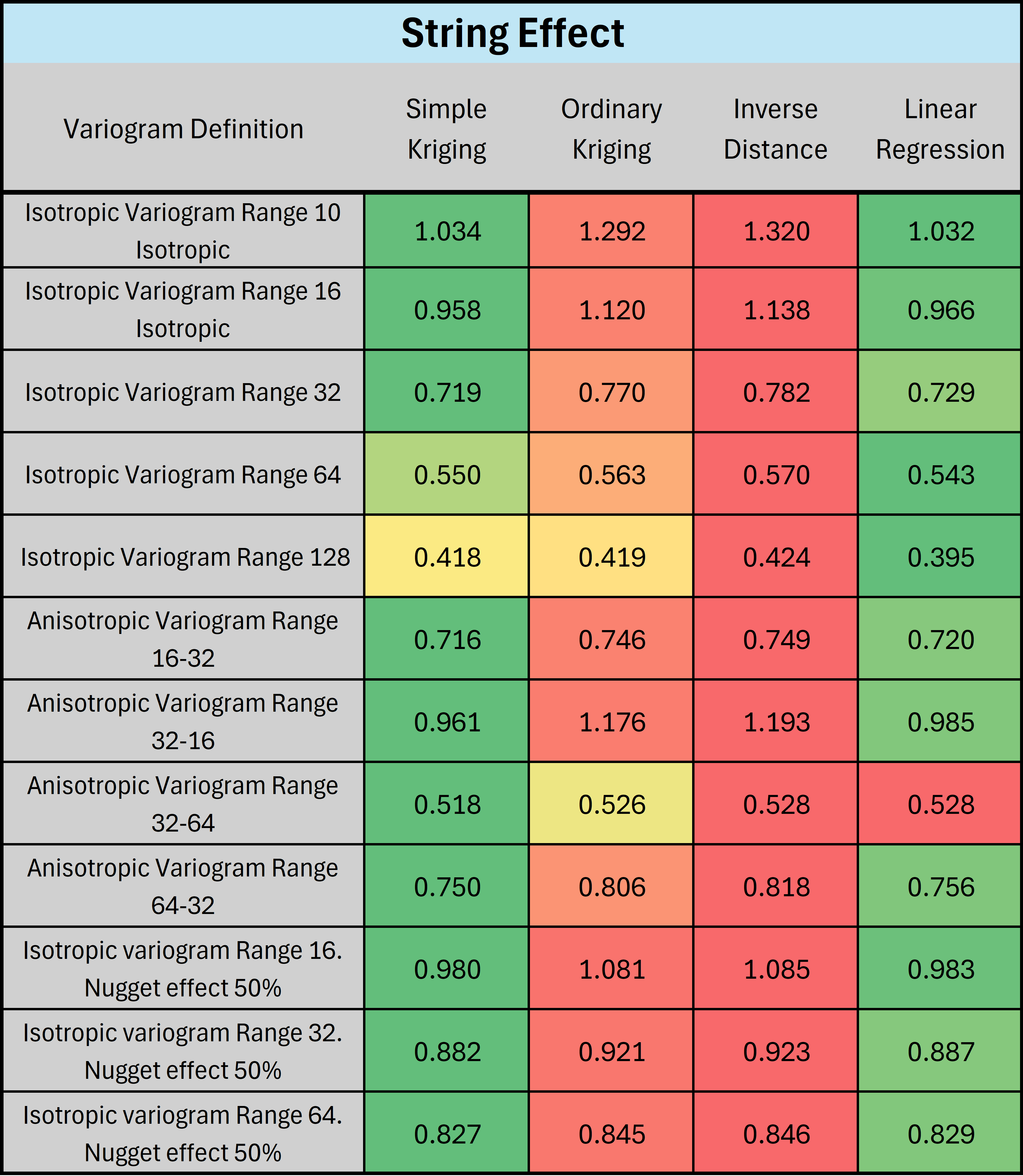
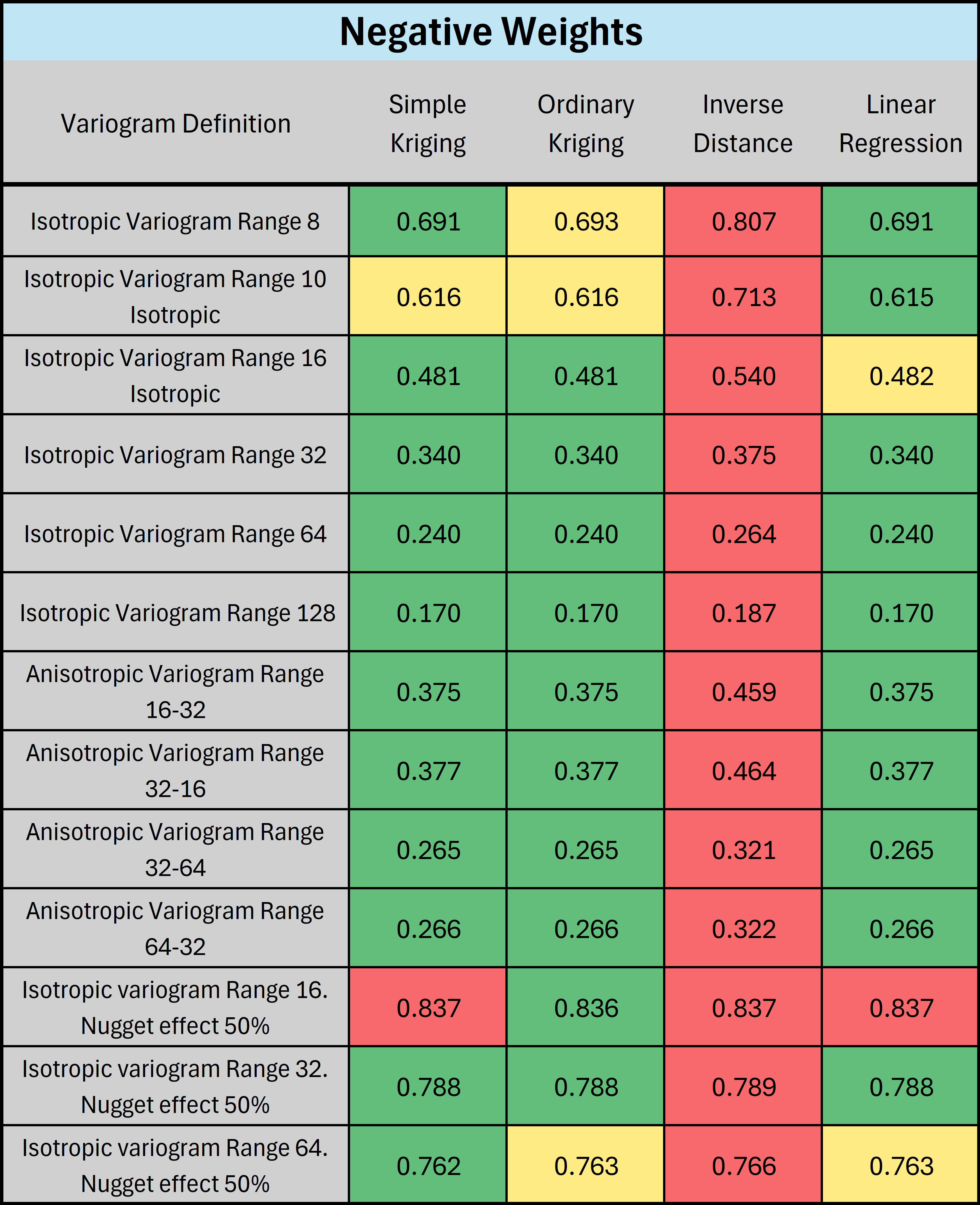
Two experiments are conducted in a stationary setting to test the optimality of kriging weights. While an ideal ergodic (infinitely large) setting requires a domain size three to ten times the largest variogram range, these experiments are conducted on a finite grid of 128 by 128 and 250 by 250. The variogram ranges span from 10 to 128 and some may not be considered ergodic by conventional standards. The first experiment compares SK, OK and inverse distance weight estimation techniques in a string effect and negative weight data configuration on a 128 by 128 simulated grid of data. The estimations are carried out at every grid location and compared to the real values. The experiment is run with changing isotropic, anisotropic and nugget effect variogram properties.

The first table summarizes the results of Experiments 1 and 2 for the string effect configuration, while the second table presents the results for the negative weight configuration. Results are displayed using the root mean squared error (RMSE) where lower values indicate better performance. SK outperformed the other estimation techniques in almost all configurations.

Experiment 2

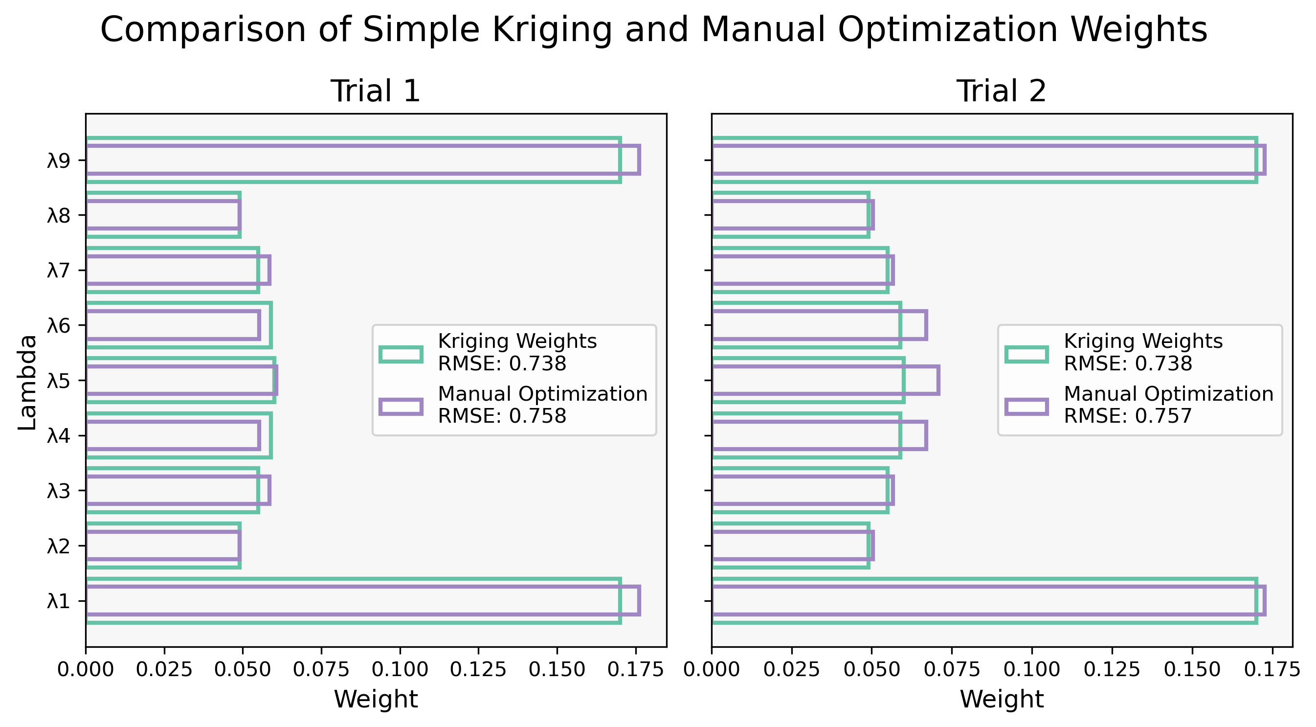
This experiment optimizes weights and compares them to SK weights in the string effect configuration. Two realizations of data are generated on a 250 by 250 grid, each realization is transformed into tabular form in two orientations: the original and a flipped version. This ensures no notion of “up or down” artifacts, allowing the results to be stationary and symmetric. \(\boldsymbol{\lambda}_1\) through \(\boldsymbol{\lambda}_9\) are initially set to \(\boldsymbol{1/9}\). A \(\boldsymbol{\lambda}\) is randomly selected and perturbed by a factor between 0.8 and 1.2. The RMSE is calculated for the entire table with the new lambda. If the error is lower, the new lambda is kept; otherwise, the original lambda is retained. This loop is performed 200,000 times then repeated with a step size of 0.99 to 1.01 to refine the weights. The experiment is run 8 times to ensure reproducibility. The manually optimized weights are nearly identical to SK. Discrepancies are reported at the second or third decimal place. Figure 3 displays results from trials 1 and 2.

These two experiments collectively demonstrate the optimality and correctness of kriging weights through different approaches:

1. Experiment 1 compares kriging methods with other traditional weighting methods. Results show SK weights are optimal in both string effect and negative weight data configurations.
2. Experiment 2 compares manually optimized weights with SK weights. Results prove kriging weights are near-optimal solutions for minimizing error variance.

The string effect and negative weights are mathematically correct and proved optimal. However, practical circumstances exist where these counterintuitive weights can cause issues for geostatistical estimation and require mitigation.

Mitigating Counterintuitive Weights

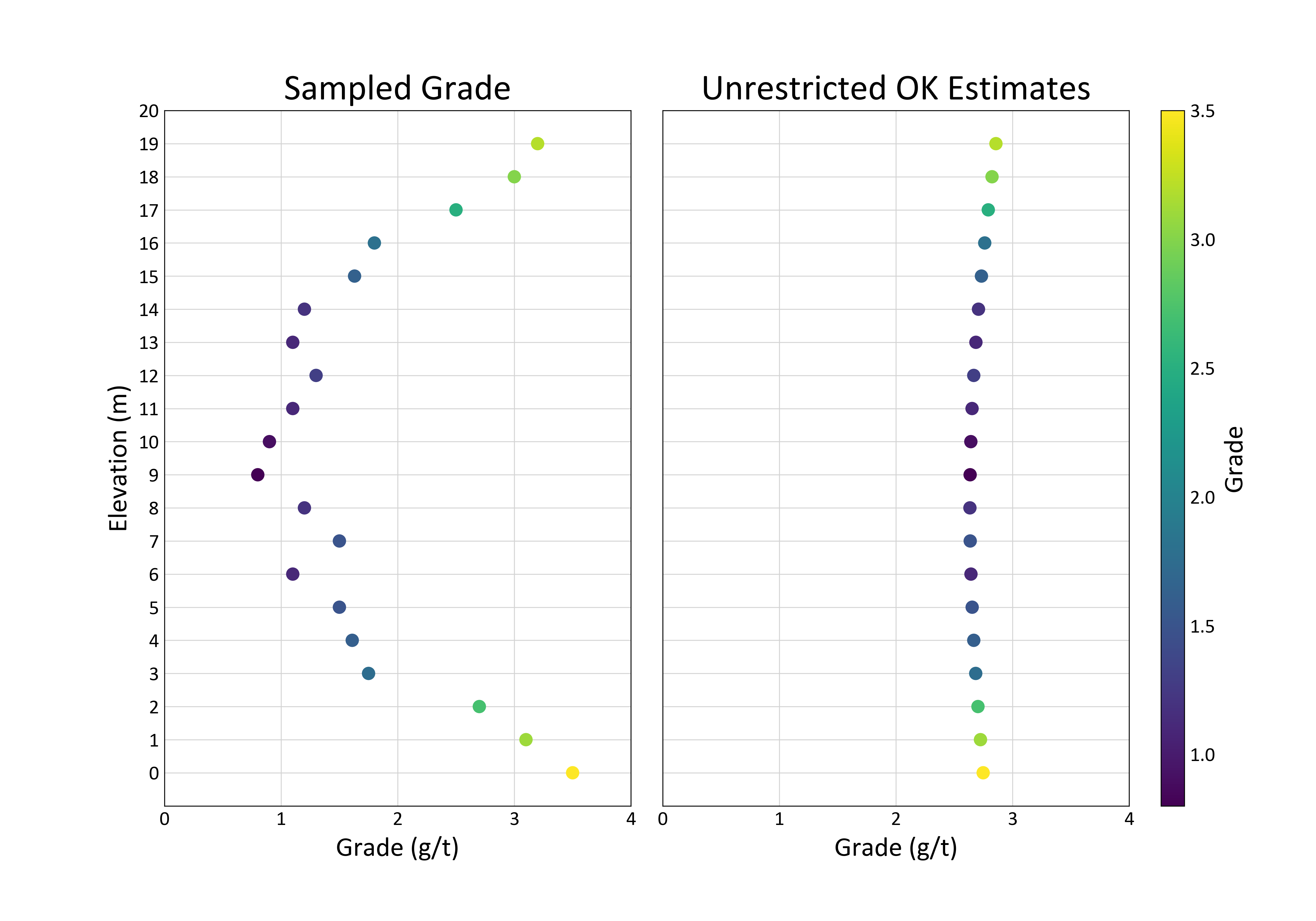
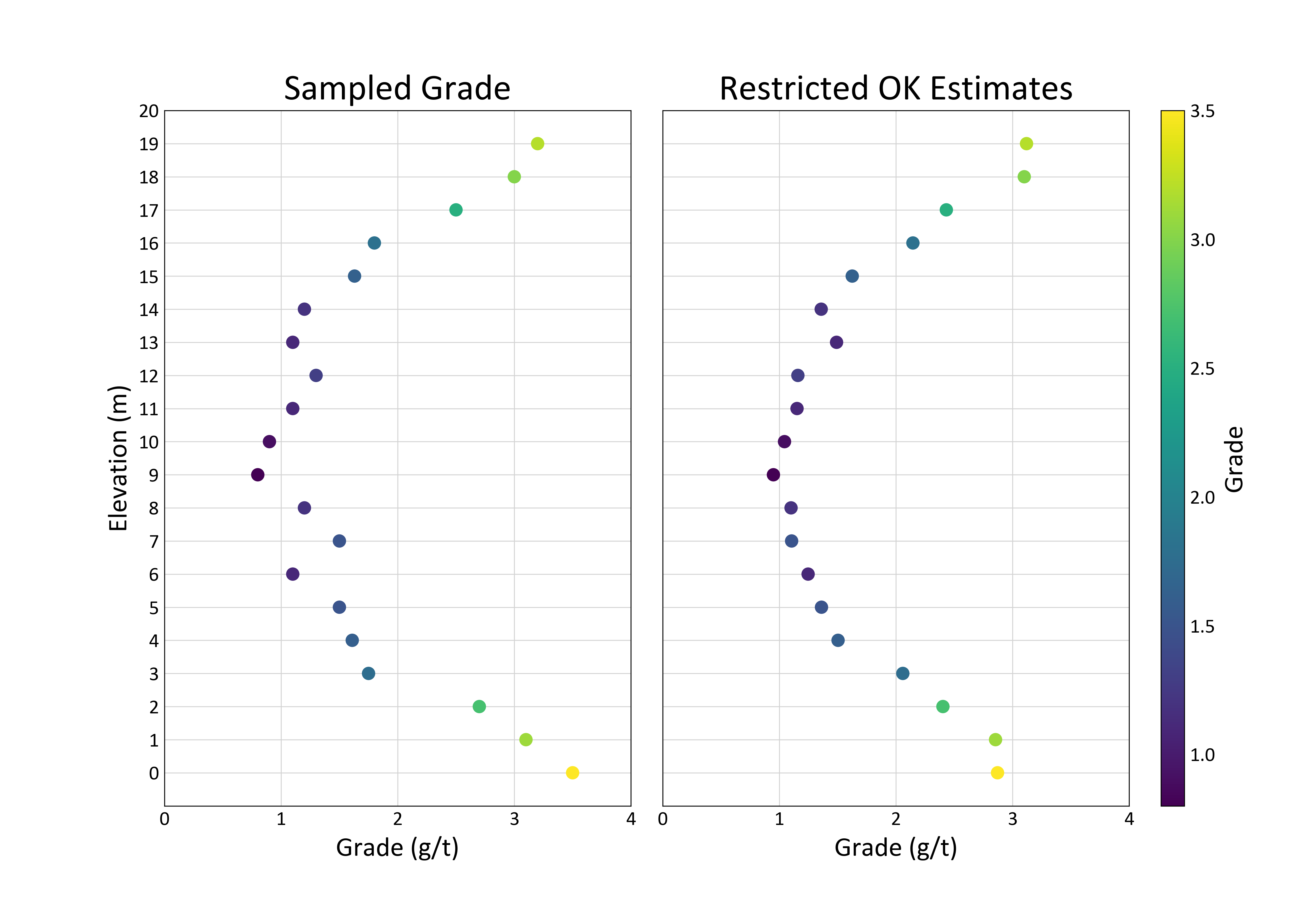
The string effect can lead to overestimation or underestimation bias in a resource estimate. An example where the string effect could lead to overestimation is described in the following scenario. High grade frequently lies at geological boundaries within mineral deposits, which are often used to define stationary domains. The string effect assigns high weights to the contact samples resulting in overestimation. Figure 4 illustrates a simplified scenario where the string effect causes overestimation bias in the center of the string with unrestricted OK. The behaviour of the bias will change depending on where the low and high grade exist or in the presence of a trend.

Two steps are taken to mitigate this consequence of the string effect.

1. Composite the drillhole appropriately.
2. Limit the number of samples per drillhole to 2 or 3

Figure 5 demonstrates the effect of restricting the OK search by limiting the number of samples used per drillhole to three. The estimate is less smooth, and the samples at the contact do not bias the estimate at the center of the domain.

Negative weights are also mathematically correct and allow for extrapolation of trends and features of data. Without them, it would be impossible to estimate above or below data limits (Deutsch, 1996). Solving the kriging equations does not constrain the estimate to be above zero. This is acceptable for some unbounded variables (e.g., normal scores or elevation), but it is not feasible for physical variables (e.g., grade or thickness).

Three options for mitigating negative weights include:

1. Constrain negative grade estimates by resetting them to zero after the fact. This method is mathematically correct and provides the closest plausible best estimate.
2. Limit the search radius. Generally, to an effective range or 2 to 3 data spacings.
3. Limit the number of data used per estimation, either total or by octant, limiting the number of screened data used per estimation.

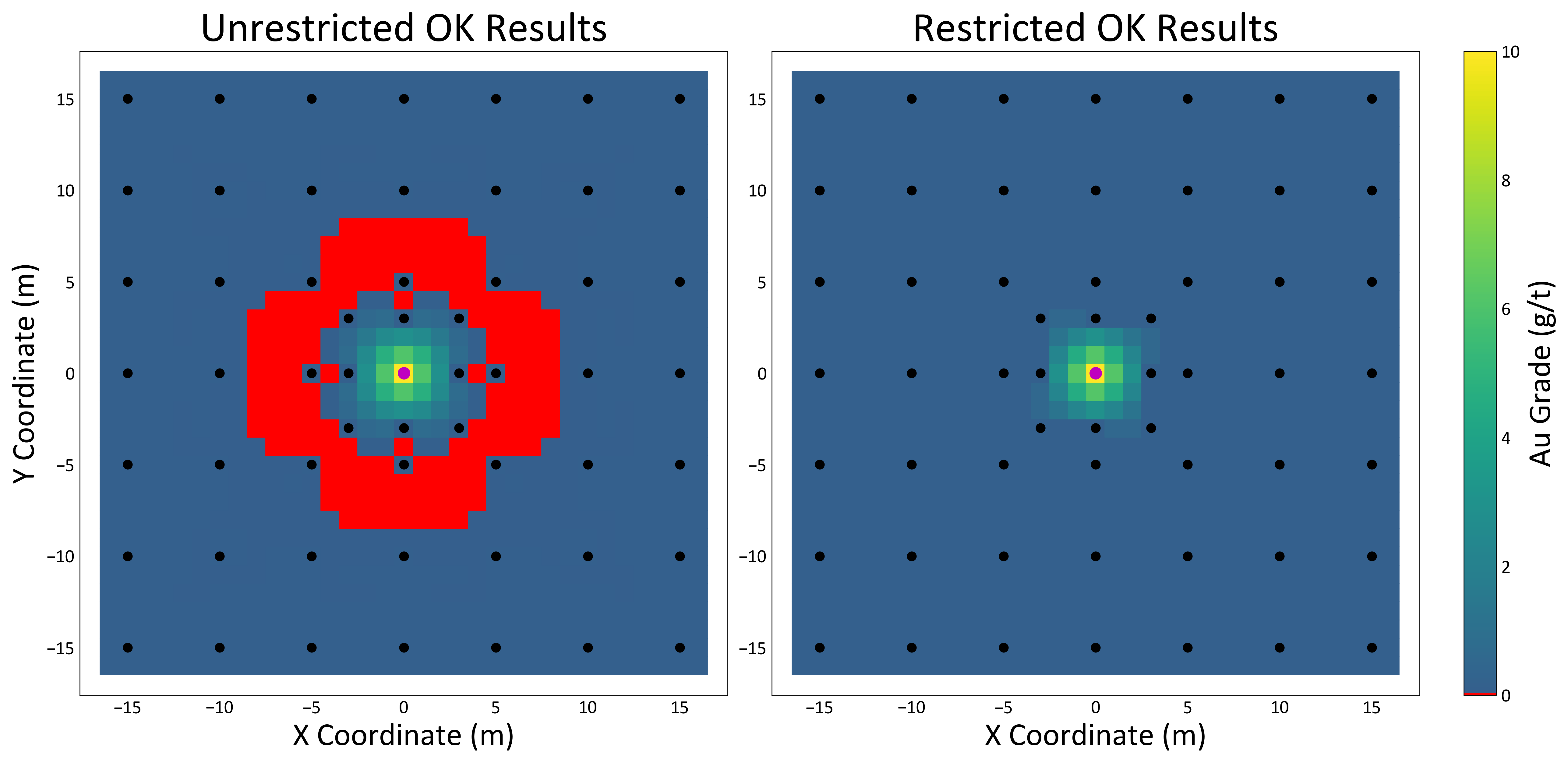
Figure 6 compares unrestricted and restricted OK results. The purple dot in the center represents a high grade sample and the black dots represent low grade samples. All estimation results below zero are displayed in red. In this data configuration the high grade sample can cause negative grade estimates when using an unrestricted search. In this example, restricting the OK search to 1 sample per octant mitigates the issue of negative estimates.

Restricting the search in an ideal stationary ergodic setting would increase RMSE from 1 to 5% versus a large search embracing the string effect and negative weights. In practice, however, it is important to keep in mind that real geologic settings are neither stationary nor ergodic.

Discussion

This lesson explores the intricacies of kriging, the current optimal geostatistical method for assigning weights to data when estimating at unknown locations. Through a series of experiments, the correctness and optimality of kriging weights are validated. The experiments highlight the superiority of kriging over traditional weighted estimation methods, and the optimality of kriging weights.

Despite their mathematical correctness and optimality, counterintuitive weights like the string effect and negative weights can pose practical challenges. The string effect may lead to overestimation or underestimation bias in circumstances where high grade or low grade occurs at geological boundaries within mineral deposits. This necessitates mitigation strategies such as appropriate compositing and limiting the number of samples per drillhole. Negative weights, while mathematically correct, can result in impossible negative estimates for physical variables like grade or thickness. Mitigation strategies include resetting negative estimates to zero, limiting the search radius, and restricting the number of data points used per estimation.

While kriging remains a powerful and reliable method for geostatistical estimations, understanding how weights are calculated and addressing the implications of counterintuitive weights are crucial for its effective application in practical scenarios. The methodologies and mitigation strategies discussed provide a framework for producing accurate kriging estimates in various geostatistical contexts.

References