Cite this lesson as: Silva, D., & Deutsch, C. V. (2026). Categorical Simulation by Truncating Gaussian Random Fields. In J. L. Deutsch (Ed.), Geostatistics Lessons. Retrieved from http://www.geostatisticslessons.com/lessons/htpgtheory
Categorical Simulation by Truncating Gaussian Random Fields
Diogo Silva
Resource Modeling Solutions
Clayton V. Deutsch
University of Alberta
July 9, 2026
Learning Objectives
- Understand the simulation of categorical variables from underlying continuous fields
- Review truncated pluri-Gaussian simulation concepts and theory
- Introduce hierarchical truncated pluri-Gaussian (HTPG)
Introduction
Categorical variables are the main control on the distribution of continuous variables (Rossi & Deutsch, 2013) and the greatest source of risk (Snowden, Glacken, & Noppe, 2002) in mining projects. There are several methodologies available for the modeling of categorical variables. These techniques can be divided into stochastic and deterministic. An important stochastic method for the simulation of categorical variables is Truncated pluri-Gaussian simulation (TPGS). Underlying Gaussian (or latent) variables are used for the simulation. These latent variables can be modeled with any one of the established methods for simulation of Gaussian random functions (GRFs). The mapping between the categorical and continuous variables is realized by truncation rules. These truncation rules allow for the introduction of modeling constraints based on geological relationships.
TPGS is a powerful method for the simulation of categorical variables, however, its application is limited to no more than three Gaussian latent variables. The hierarchical truncated pluri-Gaussian (HTPG) (Silva, 2018) simulation method was developed to facilitate the use of higher dimensionality of the latent space and therefore facilitate the modeling of more complex geological settings.
Truncated Gaussian Simulation
The simplest form of the truncated Gaussian method is the univariate case where only one latent variable is used. This form is referred to as the truncated Gaussian simulation (TGS) method and was proposed by Georges Matheron et al. (1987). A single latent variable is simulated and then truncated to define the categorical variable.
An example of TGS is shown in Figure 1. This is an 1D (location, \(\pmb{\mathrm{u}}\)) illustrative example where one realization of the latent variable \(Y(\pmb{\mathrm{u}})\) (blue line) is shown. This realization is then truncated by thresholds (two black horizontal lines \(t_1\) and \(t_2\)) defining regions that match the categories of the categorical variable. When the latent variable is below \(t_1\) the resulting category is represented by the green color. When the latent variable is between the two thresholds the resulting category is represented by the blue color, and when the latent variable is above \(t_2\) the resulting category is represented by the pink color.
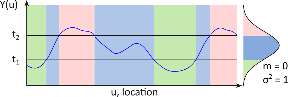
The marginal distribution of the latent variable is shown on the right side of Figure 1. Latent variables are simulated with a univariate standard normal distribution. Note that the thresholds define regions under the Gaussian bell shape for each category effectively mapping the continuous to the categorical space. The accumulated probabilities in those regions relate to the proportion of each category. The thresholds are defined based on the categorical proportions that are being targeted. If there are conditioning data, then the latent variable must fall in the correct continuous region and the category at the data location will be reproduced.
More details on the parameterization of the truncated Gaussian method and the definition of conditioning data will be discussed below. It is clear, however, that using a single latent variable is very limiting with regards to the complexity of the geological settings that can be represented. More latent variables are needed to model more realistic complex cases. This motivated the extension of the TGS method to the multivariate or pluri-Gaussian case.
Higher Dimensionality
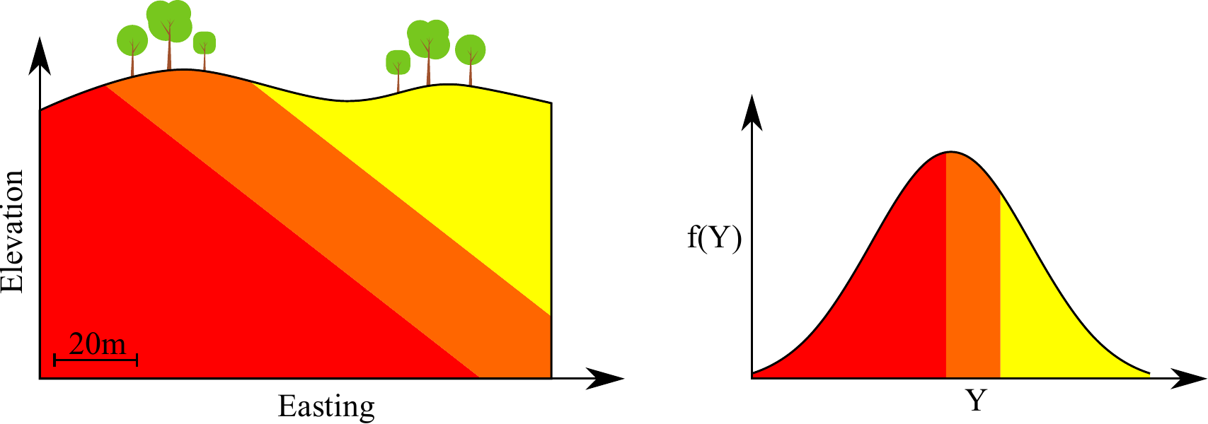
One latent variable is adequate to represent ordered layers with similar anisotropy without any discordant feature. An example of such a simple geological setting is given in Figure 2 below. Additional Gaussian variables and more complex truncation rules are required for increasing geological complexity. If an intrusion is added to the example shown in Figure 2, then an extra Gaussian variable is required to represent the discordant feature (Figure 3). In this case, the representation is simple enough and easily visualized with the bivariate truncation mask.
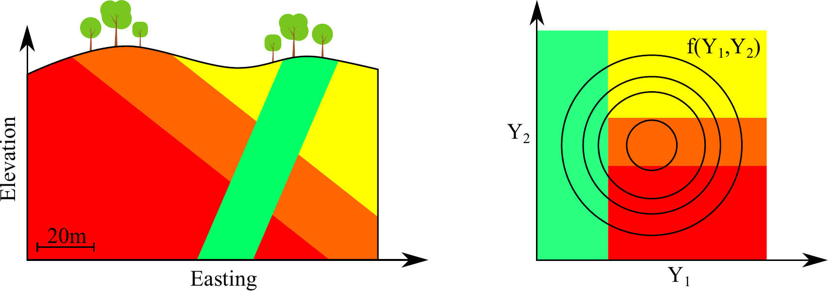
The first Gaussian variable \(Y_{1}\) is responsible to separate the intrusion from the layered categories and will control the spatial structure of the intrusion. This can be inferred from the threshold line that separates the intrusion region from the layered region. That threshold is orthogonal to the \(Y_1\) axis. The second Gaussian variable \(Y_{2}\) controls the spatial structure of the three layered categories. The spatial structure of the two sets of categories is not mixed because the thresholds are orthogonal with relation to the Gaussian variables.
More Gaussian variables are required if additional geological complexity is added. In Figure 4, an additional discordant structure is added, that is, an erosional surface is included with additional depositional layers on top of it.
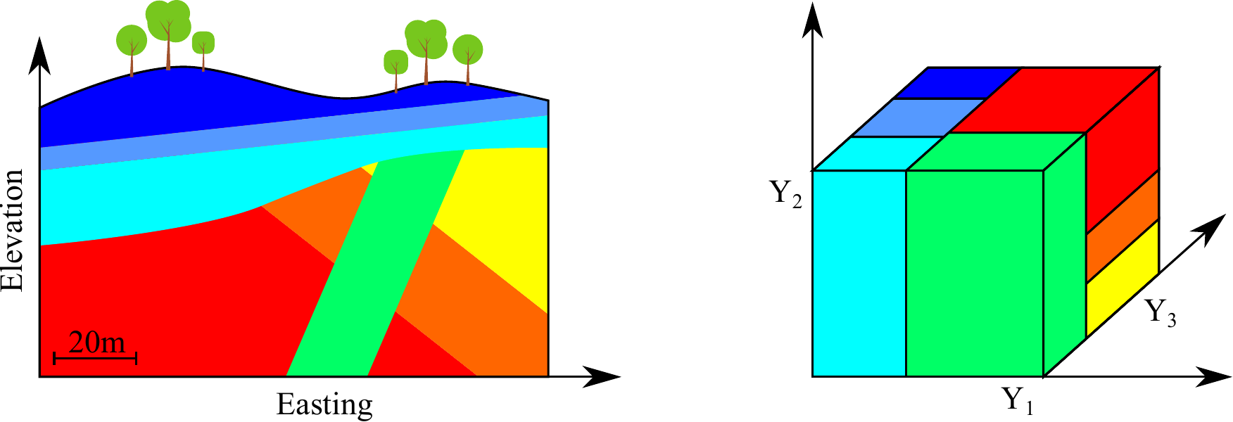
At first glance, one would think that one additional Gaussian variable would suffice to represent the geology. In that case a bivariate truncation mask could be created as shown in Figure 4. The Gaussian variable \(Y_{1}\) controls the transition between the structures above the erosional surface and the structures below ensuring that they do not cut through that boundary. The Gaussian variable \(Y_{2}\) controls the transition between the layers below the erosional surface. The Gaussian variable \(Y_{3}\), however, controls the transition between the layers above the erosional surface and the transition between the intrusion and the layers below the erosion. Given that these two structures have different spatial structure (direction and shape), the truncation mask shown in Figure 4 does not represent the geological setting that is shown.
Another alternative truncation mask is shown in Figure 5. For this example, \(Y_{1}\) controls the transition between the layers on top of erosional surface. \(Y_{2}\) controls the transition between the layers below the erosional surface. The Gaussian \(Y_{3}\) controls the spatial structure of the intrusion. This mask separates each geological unit’s spatial variability utilizing an independent Gaussian variable, however, this setting still allows for the intrusion to cut through the layers above the erosional surface. At least four Gaussian variables are required to properly account for all the shapes and boundary constraints shown in this example. An easy visualization and geological interpretation of the historical bivariate or trivariate truncation mask is not possible for this example.
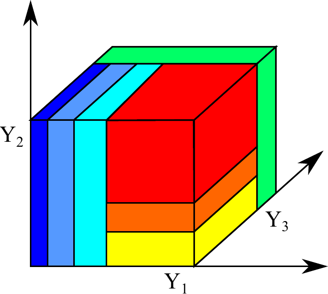
There are alternatives to the historical truncation rules available for utilization with higher dimensions. J. L. Deutsch & Deutsch (2014) proposed multi-dimensional scaling (MDS) to generate masks by Voronoi decomposition of a multivariate space. The technique is data driven and removes the opportunity to add geological expert knowledge to the truncation rule. In addition, the boundaries of the truncation regions are not orthogonal to the variable axes, resulting in the mixing of spatial structures and making it more difficult to map the spatial structure of the latent variables to the categorical space.
Another approach is proposed by Madani & Emery (2015). The truncation rule is represented by a simple binary tree with a linked list structure where each node is used to segregate one category. The HTPG can be seen as a generalization of this technique where more complex tree structures are allowed depending on the geological structure observed. The technique proposed in Madani & Emery (2015) represents a case where the categories show minimum spatial structure.
Hierarchical Truncated pluri-Gaussian (HTPG) Simulation
Before HTPG most applications of TPGS were restricted to two dimensional truncation rules mostly because the geological interpretation of the historical truncation rules in higher dimension is difficult. The increased difficulty of mapping the spatial variability of the categorical variable to the continuous space is often used to justify the restriction to the bivariate case (Armstrong et al., 2011).
The idea of using hierarchical rules with larger number of latent variables to model multiple categories precedes the development of the HTPG framework. The binary tree structure proposed by Madani & Emery (2015) is one example, however, binary truncations cannot represent all possible geological structures. HTPG can be seen as a generalization of this technique in which more complex tree structures can be used to describe the contact relationships between geological domains. This allows for more flexibility in what can be represented.
The geology represented in Figure 4 is conceptualized again in Figure 6. The template represents the geology due to a set of geological events. Categories 5, 6 and 7 were deposited in ordered layers which were tilted from its original horizontal orientation. The category 4 can be interpreted as a dike that came later cutting through categories 5, 6 and 7. The resultant sequence was later eroded and categories 1, 2 and 3 were deposited in layers on top of the erosional surface.
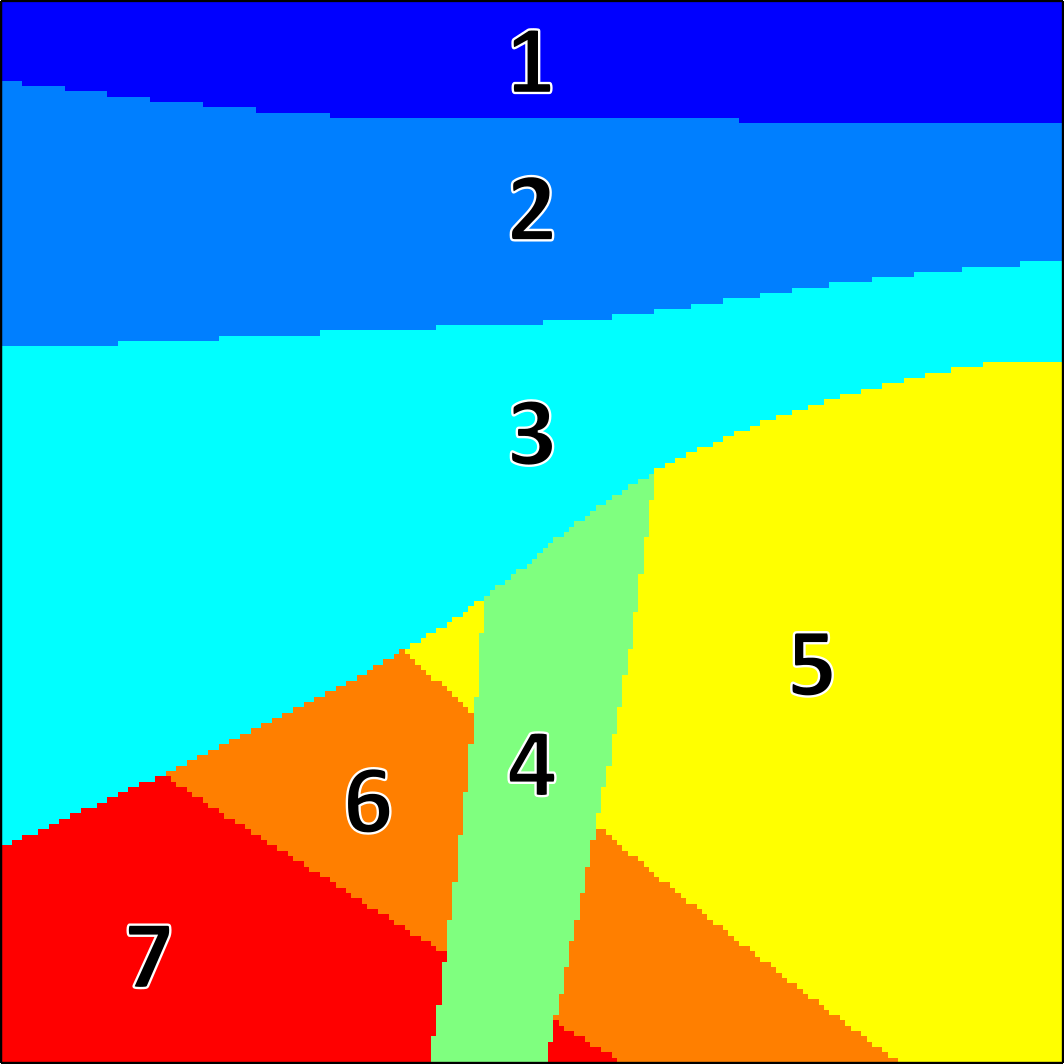
The truncation rule in HTPG is defined by a decision tree structure. Every parent (non-leaf) node on the tree structure represents a Gaussian latent variable. The parent nodes are also where the thresholds are applied. The leafs of the tree are the resulting categories. There can only be one leaf per category. This entails that there are only \(B-1\) thresholds and that the number of Gaussian variables must be less or equal to the number of thresholds. \(B\) is the number of categories which is 7 in this illustrative example.
The geological setting shown in Figure 6 is complex enough to make alternative truncation masks unworkable, however, the definition of a truncation rule is quite straightforward with a hierarchical tree structure. The geological setting can be reconstructed with a hierarchical set of truncation rules defined by the tree structure shown in Figure 7.
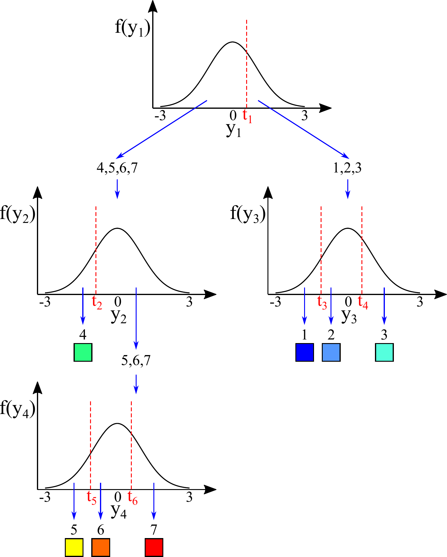
Four Gaussian variables are required to represent this geological setting. The first Gaussian variable (\(Y_{1}\)) defines the erosional surface that separates the categories 1, 2 and 3 from the categories 4, 5, 6 and 7. The Gaussian variable \(Y_{2}\) separates the discordant category 4 from the layered categories 5, 6 and 7. The Gaussian variable \(Y_{3}\) separates the layered categories 1, 2 and 3. Finally the Gaussian variable \(Y_{4}\) separates the layered categories 5, 6, and 7.
This simple example illustrates how one can define hierarchical truncation rules using multiple Gaussian variables to define the transitions and ordering between different categories. This simple exercise of defining geologically sound truncation rules for this many latent variables and categories would have been much more difficult without the hierarchical tree structure. The hierarchical procedure can be easily used to separate (1) sets of categories that do not belong together such as sets of rocks types separated by erosional surface, (2) cross cutting (discordant categories) such as intrusive rocks, (3) ordered categories such as sedimentary sequences, and (4) background categories.
The truncation structure to use with HTPG may not be clear in cases where there is not enough confidence in the geological understanding. This may be the case in early stages of projects or due to sparse drilling that may be common for some commodities. Sanchez (2023) explored ways to define multiple possible classification trees as well as score metrics to evaluate their performance and assist in the definition of an appropriate set of parameters for HTPG truncation rules.
The typical workflow steps for the application of HTPG are outlined below. Upstream steps such as parameter uncertainty and downstream steps such as the use in multivariate continuous property modeling are not covered here. The steps for HTPG:
- Prepare data and determine anisotropy
- Model trends of categorical variable proportions
- Perform indicator residual variography
- Specify truncation tree
- Derive latent variable variograms
- Impute realizations of latent variable at data locations
- Check imputed data distribution
- Check imputed data spatial continuity
- Simulate and truncate realizations of latent variables
- Check latent simulated realization’s distribution
- Check latent simulated realization’s spatial continuity
- Check and post-process categorical realizations
- Check reproduction of global proportions
- Check reproduction of indicator variograms
- Calculate probabilities and entropy
HTPG Parameterization - Defining Thresholds
HTPG thresholds and categorical proportions are closely related; the thresholds are increased and decreased as necessary to get the correct proportions. The Equation below shows the relation between thresholds of the \(i_{\text{th}}\) category and its proportion (\(p_i\)). The thresholds \(t^{(i,j)}_{\text{min}}\) and \(t^{(i,j)}_{\text{max}}\) represent the bounding thresholds of the \(j_{\text{th}}\) latent variable (\(y\)) for the \(i_{\text{th}}\) category and \(\Phi\) is the standard normal cumulative distribution function (CDF).
\[ p_{i} = \prod_{j=1}^{K} \left[ \Phi \left({y_j}{\le}t_\text{max}^{(i,j)}\right) - \Phi \left({y_j}{\le}t_\text{min}^{(i,j)} \right) \right] \qquad \forall i \in \{1,\ldots,B\} \qquad \text{(1)} \]
To illustrate this calculation we can consider category 2 from Figure 7. All thresholds for category 2 are shown in Table 1. The resulting term in the multiplier shown in Equation 1 is 1.0 for all cases where the minimum and maximum thresholds are \(-\infty\) and \(+\infty\). The final proportion for category 2 is then defined by \(p_2 = [1.0-\Phi(t_1)] \times [\Phi(t_4)-\Phi(t_3)]\).
| Latent Variable | \(t_{\text{min}}\) | \(t_{\text{max}}\) |
|---|---|---|
| \(Y_1\) | \(t_1\) | \(+\infty\) |
| \(Y_2\) | \(-\infty\) | \(+\infty\) |
| \(Y_3\) | \(t_3\) | \(t_4\) |
| \(Y_4\) | \(-\infty\) | \(+\infty\) |
| \(Y_5\) | \(-\infty\) | \(+\infty\) |
| \(Y_6\) | \(-\infty\) | \(+\infty\) |
| \(Y_7\) | \(-\infty\) | \(+\infty\) |
In practice, the deemed representative proportions from data, should be reproduced quite closely. The domains control the mineralization and therefore the tonnage of resources. The proportions can be calculated globally with declustering weights. The equation for calculating thresholds from the categorical proportions:
\[ t_{j} = \Phi^{-1} \left( \frac{ \sum\limits_{ i {\in} \mathcal{B}_{k,j} } p_i } { \sum\limits_{ i {\in} \mathcal{B}_{k} } p_i } \right), \qquad \forall j \in \{1,\ldots,B-1\} \qquad \text{(2)} \]
where \(\mathcal{B}_{k}\) is a subset of \(\mathcal{B}\) with all the categories that are relevant to the node \(k\) (or latent variable \(Y_{k}\)) where the threshold \(t_{j}\) is applied. \(\mathcal{B}_{k,j}\) is a subset of \(\mathcal{B}_{k}\) with all the categories that are defined below the threshold \(t_{j}\).
To calculate the threshold \(t_6\) (from Figure 7), for instance, we need to first identify the variable or node where it is applied: that is, \(Y_4\). Then, find all categories that are defined in that node (5, 6 and 7) and the categories that are below \(t_6\) (5 and 6). In this case the threshold \(t_6\) is calculated from the category 5, 6 and 7 proportions by \(t_6 = \Phi^{-1}\left(\frac{p_5 + p_6}{p_5 + p_6 + p_7}\right)\). Note that with local proportions defined at locations \(\pmb{\mathrm{u}}\) we can apply the same equation where we have local proportions \(p_i(\pmb{\mathrm{u}})\) \(\forall i \in \{1,\ldots,B\}\) and get local thresholds \(t_j(\pmb{\mathrm{u}})\) \(\forall j \in \{1,\ldots,B-1\}\). All these calculations are performed by the software.
Non-Stationarity
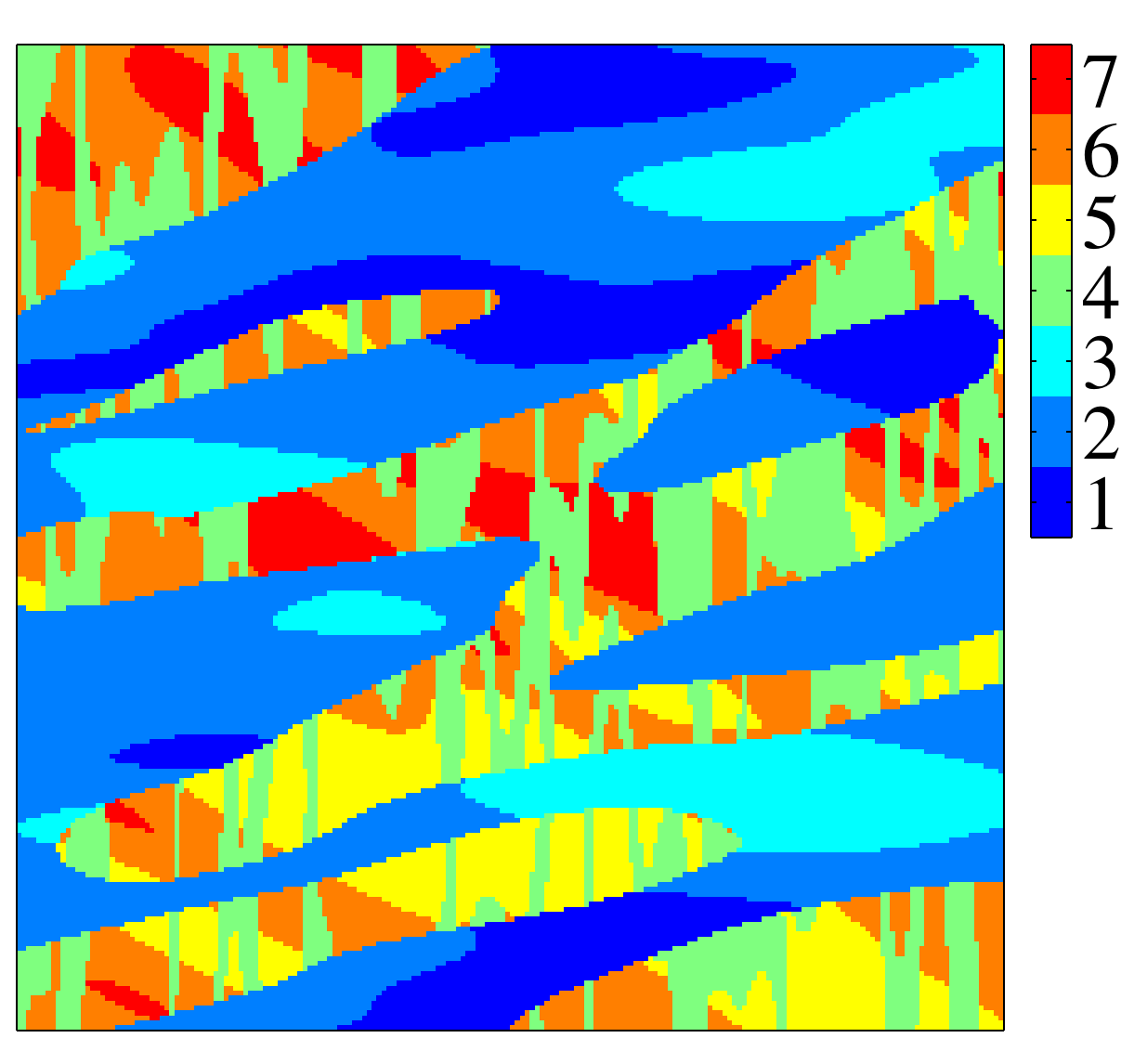
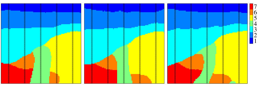
Categorical variables that represent geological settings are rarely stationary in nature. The geological setting shown in the conceptual model Figure 6 without any consideration of non-stationarity could yield the categorical realization shown in Figure 8. This model shows many of the correct features such as ordered layers for categories 1, 2 and 3 and also 5, 6 and 7, as well as the cross-cutting dike (category 4). Categories 4, 5, 6 and 7 at the top (where only categories 1, 2 and 3 are expected) is incorrect. The same happens for category 1, 2 and 3 that appear at the bottom. There are also symmetric transitions instead of the expected asymmetric transitions from the conceptual model. For instance, going from the top to the bottom, we should only see transitions from 3 to 2 to 1, but we also see 1 to 2 to 3. The same can be said for categories 4, 5 and 6. This is expected as the GRF that we are simulating is stationary and symmetric.
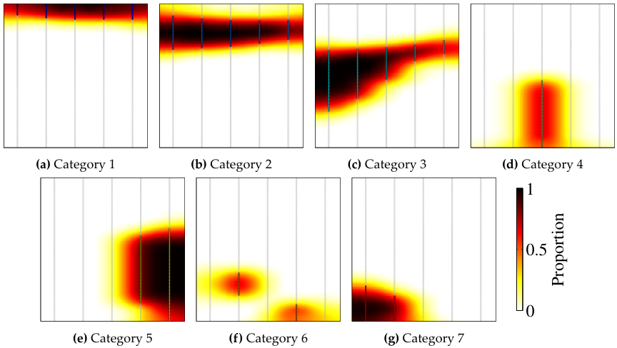
Local proportions (categorical trends) are calculated with moving window averages (MWAs) applied to indicators. The process for trend calculation is similar to what is done for continuous variables (Harding & Deutsch, 2021; Qu & Deutsch, 2018). Trend models for categorical variables must be used to define local thresholds. A trend model constructed with a MWA applied to samples extracted from the 2D model from Figure 6 is shown in Figure 9. These local proportions are sufficient to enforce the non-stationarity and asymmetry observed in our data and conceptual model on our final realizations (Figure 10).
Latent Variable Variograms
All truncated Gaussian techniques require the modeling of GRFs to serve as underlying latent variables for the definition of categorical models. This requires the definition of the spatial correlation model for the Gaussian latent variables. In practice, only the indicator variograms of the categorical variable can be calculated. The matching spatial structure in continuous space has to be defined to ensure the reproduction of the categorical spatial continuity. The indicator variogram cannot be used directly for the latent variables (Kyriakidis, Deutsch, & Grant, 1999; G. Matheron, 1989). Note that if local proportions are being considered, then the variogram of the indicator residual (Equation 4) should be used instead.
\[ r_{ij} = I_{ij} - p_{ij} ,\qquad \forall i \in \{1,\ldots,n\}, \quad \forall j \in \{1,\ldots,B\} \qquad \text{(4)} \]
where \(r_{ij}\) is the residual, \(I_{ij}\) is the indicator and \(p_{ij}\) is the proportion for the \(j_\text{th}\) category at \(i_\text{th}\) data location.
The most practical solution to this problem is to apply a numerical inversion approach to calculate the spatial continuity in continuous space that maps to the categorical space. The procedure used in the HTPG framework is based on the numerical approach proposed by Zagayevskiy & Deutsch (2015). This approach can be applied to any type of truncation rule. The technique is adapted to HTPG and further developed to enhance its computational efficiency and practicality.
The goal of the numerical derivation is to define the variogram model of the Gaussian latent variables that generates realizations of the categorical variable with indicator variograms that are as close to the modeled indicator variograms as possible. This is achieved by an inversion algorithm that utilizes a Monte-Carlo simulation (MCS) (Silva, 2018) framework coupled with a line search optimization.
Figure 11 shows an illustration of the MCS based inversion algorithm being applied to the fourth node of the lag discretization. The variograms of the latent variables (left side) are unknown. The first three nodes have been defined before the illustrated state. The lower limit for the line search is the optimized variogram value for the previous lag distance. The upper limit is always 1.0. The yellow markers show the iteration points and the green is the final optimum. Each node have its counterpart on the categorical indicator variograms shown on the right side. The red lines are the reference indicator variogram models. The mismatch between the nodes and this line is minimized.
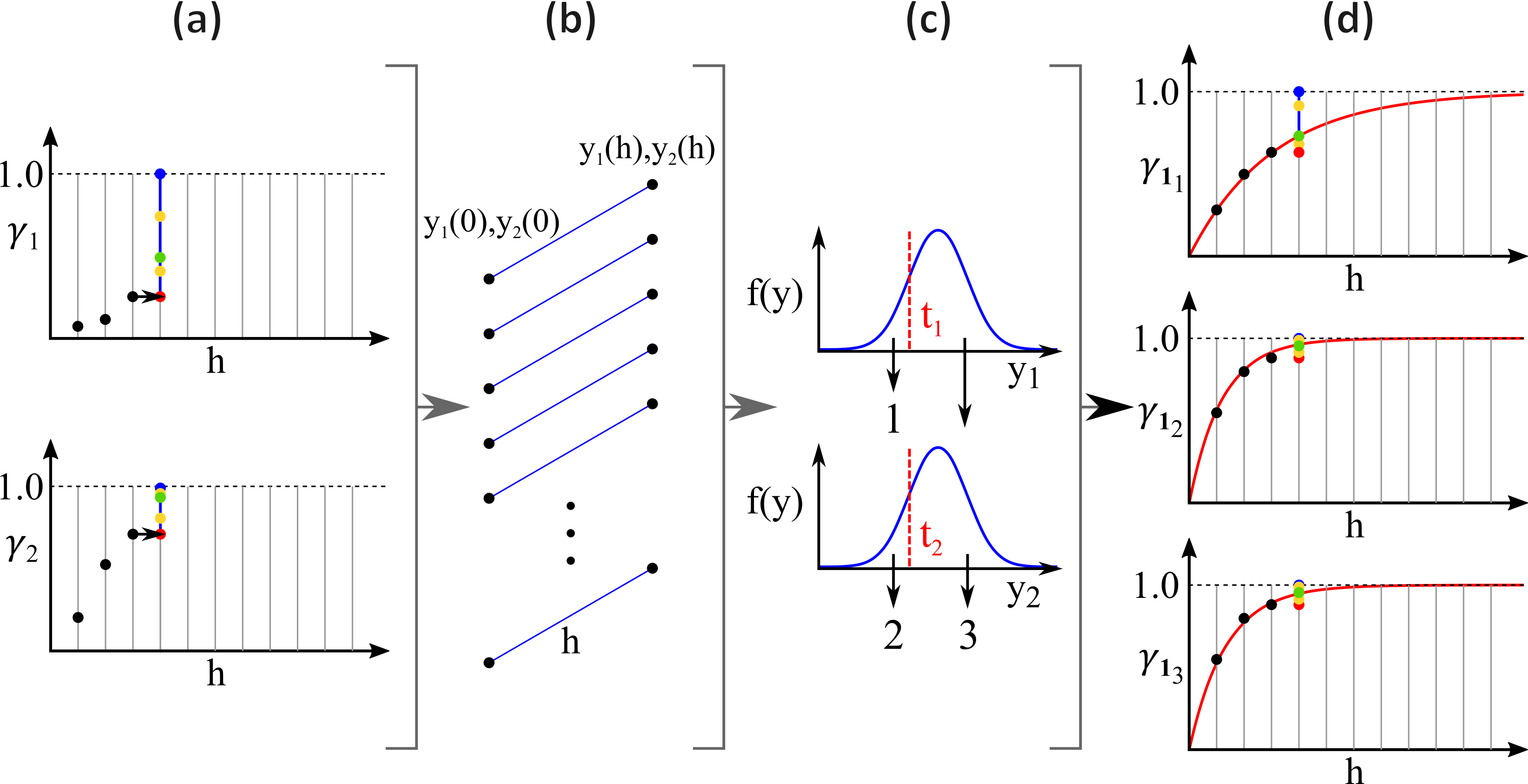
To map a latent variable variogram (left side) value for a given lag (\(\gamma(\pmb{h})\)) to the categorical variogram (right side) a large number of data pairs in latent space correlated by \(\rho(\pmb{h}) = 1 - \gamma(\pmb{h})\) is randomly generated and then the truncation rule is applied to define the categorical observations that are finally used to calculate the indicator variogram on the right side for the selected lag vector.
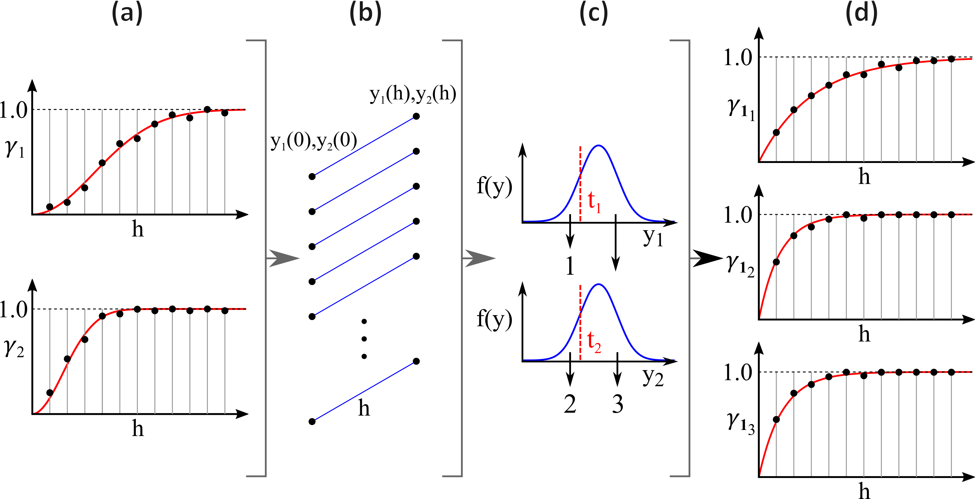
An illustration of the final state of the numerical derivation is shown in in Figure 12. After all nodes are optimized, the variogram of the latent variables (left side) are fitted with valid variogram models (red lines). The nodes on the right side indicates the expected reproduction of the reference indicator variograms (red lines). If the optimized points are fitted well, the mapped points in the categorical space can be seem as the expected variogram reproduction of the HTPG. This numerical derivation is fully automated within the software for a given truncation rule, global proportions and input categorical variograms. Gaussian variogram structures are typically used to fit the experimental points as they are quite continuous and produce sharp boundaries between categories that is common.
Conditioning Data
The Gaussian latent variables used in truncated Gaussian techniques are a model assumption, therefore, these variables are not observed. The truncated Gaussian techniques generate realizations of these latent variables to be truncated to define the categorical models. Samples of the categorical variable are the only data available. The simulated categorical models are expected to match these data observations. If \(n\) observations of the categorical variable are available, the condition in Equation 3 must be met for all locations. That means that when we apply the truncation to the latent variables at a data location we expect it to result in the same category observed at that data location.
\[ x_{i} = \mathcal{M}_{\theta}\left(\pmb{y}_{i}\right) ,\qquad \forall i \in \{1,\ldots,n\} \qquad \qquad \text{(3)} \]
where \(\mathcal{M}_{\theta}\) is the truncation mapping parameterized by a set of parameters \(\theta\); \(\pmb{y}_{i}\) is a vector with the latent variables at location \(i\); and \(x_{i}\) is the categorical observation at the \(i_\text{th}\) data location.
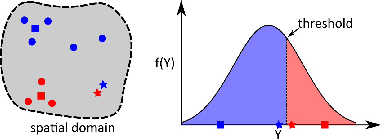
The categorical observations are soft constraints on the possible values for the latent variable at any given location, the exact values are unknown. The latent variable is spatially correlated and its spatial structure is related to that of the categorical variable. Two locations close together are more likely to have similar values than two locations far apart. Figure 13 shows an illustrative example of the effect of the spatial configuration of the categorical samples on the underlying latent variable. The star shaped samples are spatially close to each other, however, they show different categories. In this case the latent variable is expected to be near the threshold if there is spatial correlation between them. The square shaped markers are samples that are within a region surrounded by the same category. In this case, there is a low probability that the latent variable is close to the threshold, in fact, they have a higher chance to be far apart within the standard Gaussian distribution. The definition of the latent variables should account for the spatial structure and also be conditioned to the categorical data observations.
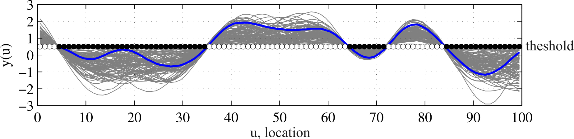
The solution to Equation 3 is non-unique. There are multiple realizations of the latent variable that satisfy the same set of categorical data observations. This is illustrated in Figure 14. The blue line is the true underlying latent variable that is not observed in practice. The black and white markers are the categorical observations, the only data available. The grey lines are multiple realizations of the latent variable that has the same spatial continuity and that satisfies the observed categorical data. To transfer the uncertainty of the unobserved latent variables, a multiple imputation framework should be utilized (Silva & Deutsch, 2019). To achieve that, each realization of the categorical variable generated with a truncated Gaussian method should utilize a different realization of the latent variable.
Sampling directly from a high-dimensional truncated Gaussian distribution is not feasible, however, sampling from the marginal univariate conditional distributions is simple. The Gibbs sampler method is well suited for the task of indirectly generating samples of a complex multivariate distribution utilizing the univariate conditional distributions. Variations of the Gibbs sampler algorithm for the data imputation in the truncated Gaussian methods have been developed by many researchers (Astrakova, Oliver, & Lantuéjoul, 2015; Emery, Arroyo, & Peláez, 2014; Galli & Gao, 2001; Geman & Geman, 1984; Lantuéjoul & Desassis, 2012).
The convergence of the Gibbs sampler algorithm is a recurring problem with the sampling of correlated variables. Care must be taken to ensure good convergence or at minimum a close enough solution in terms of spatial continuity and Gaussianity. This can be achieved by careful parameter selection and Gibbs sampler initialization algorithm.
Simulation of Latent Variables and Mapping to Categorical Space
After the latent variables are defined at data locations, they can be simulated at all nodes of the modeling grid. Any method for the simulation of Gaussian variables can be used. The most common techniques for the generating of GRF in geostatistics are the turning bands (TB)(Journel, 1974; G. Matheron, 1973), and sequential Gaussian simulation (SGS) (Gómez-Hernández & Journel, 1993; Isaaks, 1990).
Once the Gaussian variables are simulated at every grid node, the realizations are mapped back to the categorical space by applying the truncation rule. At this point, if all the preceding steps are properly applied, the categorical realizations should match the categorical data observation, the spatial structure given by the indicator variograms, the categorical proportions and transition probabilities. # Summary
This lesson reviews the concepts behind the utilization of a continuous latent variable for the geostatistical simulation of discrete categories. The hierarchical framework using the HTPG approach is described that unlocks the potential of the TPGS technique facilitating the introduction of geological expertise such as known constraints and relationships between categories into the modeling procedure. The importance of accounting for non-stationarity is reinforced as it is commonly observed in most, if not all, practical applications. Data uncertainty related to the unsampled latent variable must be quantified and carried over throughout the workflow using multiple data imputation. The simulated realizations must be validated following the best practices. Some of these validations are described in C. V. Deutsch (2017). HTPG has been applied to many deposits such as porphyries, carlin style deposits, massive sulfides and select skarns.