Learning Objectives

• Understand how to draw an error ellipse (or density contour) of a bivariate Gaussian distribution considering a given confidence level.
• Derive the equations for combining multivariate Gaussian distributions through error ellipses.
• Appreciate the error ellipses method using a simulated bivariate Gaussian dataset.

Introduction

The combination of probability distributions is a common challenge encountered in geology, engineering, and statistics. The distributions come from different data sources or sensors. The distributions could be univariate, bivariate or multivariate. The techniques to combine the distributions include (1) formulating and parameterizing a high dimensional distribution from which conditional distributions can be computed - called cokriging in geostatistics (C. V. Deutsch & Journel, 1998; Doyen, 1988) (2) considering a known prior distribution and making a neutral assumption about the redundancy in the information content - called collocated cokriging or Bayesian Updating in geostatistics (Doyen, Boer, & Pillet, 1996; Xu, Tran, Srivastava, & Journel, 1992), and (3) considering no prior distribution and conditional independence in the likelihood distributions - called Error Ellipses in the literature (Blachman, 1989). This Lesson aims to develop the latter technique.

There is a reasonably informed prior distribution in most spatial prediction problems; it comes from a careful choice of a stationary population and declustering of the available data. The error ellipses method would not be appropriate. There are situations, however, where there is no prior and the data sources are very different; the error ellipses technique is useful when the convex estimation of the probability distribution is required. For example, the horizontal variogram calculated from a few wells are highly uncertain, whereas the horizontal variogram calculated from dense seismic information would be more structured but noisier. The estimation of the horizontal variogram from the wells can be improved by combining the distributions of the squared differences from wells and seismic information for each lag (Rezvandehy, 2016). In this Lesson, the construction of the confidence ellipse of a bivariate Gaussian distribution is first reviewed. The error ellipse method and derivation of its equations are explained, and the method is demonstrated using a simulated bivariate Gaussian dataset.

Multivariate Gaussian Distribution

Probability Density Function

Consider a \(p\times 1\) random vector \(\mathbf{X}=[X_{1},...,X_{p}]^{T}\) that has a multivariate Gaussian distribution \(\mathbf{X}\sim N_{p}(\boldsymbol{\mu},\Sigma)\). Its probability density function is given as follows:

\[f(\mathbf{X}|\boldsymbol{\mu}, \Sigma)=\dfrac{1}{(2\pi)^{p/2}|\Sigma|^{1/2}} exp\left\{-\dfrac{1}{2}(\mathbf{X}-\boldsymbol {\mu})^{T}\Sigma^{-1}(\mathbf{X}-\boldsymbol{\mu})\right\}\]

where \(p\) is the dimension of the vector; \(\boldsymbol{\mu}\) is the \(p\times 1\) vector of means \(\boldsymbol{\mu}=[\mu_{1},...,\mu_{p}]^{T}\), and \(\Sigma\) is the \(p\times p\) positive definite covariance matrix \(\Sigma\) of \(\mathbf{X}\):

\[\Sigma= \begin{bmatrix} \sigma_{11} & \sigma_{12} & \cdots & \sigma_{1p}\\ \sigma_{21} & \sigma_{22} & \cdots & \sigma_{2p}\\ \vdots & \vdots &\ddots & \vdots \\ \sigma_{p1} & \sigma_{p2} & \cdots & \sigma_{pp}\\ \end{bmatrix}\]

If a random vector \(\mathbf{X}\) is multivariate Gaussian, each random variable of \(\mathbf{X}\) is also Gaussian. If \(\rho=0\), that is, \(\Sigma\) is of a diagonal matrix (all off-diagonal elements are zero), the multivariate Gaussian distribution is equal to \(p\) number of univariate Gaussian distributions (Johnson & Wichern, 1988).

Density Contours of a Bivariate Gaussian Distribution

The plot of the density (or probability) contours of a bivariate Gaussian distribution represents a three-dimensional surface. The constant probability contours, however, can be plotted on a two- dimensional format by considering the same height on the z-axis (or the constant height of the surface). Consider that a random vector \(\mathbf{X} = [X_{1}, X_{2}]\) has a bivariate \((p=2)\) Gaussian distribution. The scalar quantity of the square of the distance \((\mathbf{X}-\boldsymbol {\mu})^{T}\Sigma^{-1}(\mathbf{X}- \boldsymbol{\mu})=K\) is referred to as the Mahalonobis distance of the vector \(\mathbf{X}\) to the mean vector \(\boldsymbol{\mu}\). The surface on which the random variable \(K\) is constant is an ellipse (or a \(p\)-dimensional ellipsoid in the multivariate case) centered at \(\boldsymbol {\mu} = [\mu_{1},\mu_{2}]\). This ellipse (or a probability contour) defines the region of a minimum area (or volume in multivariate case) containing a given probability under the Gaussian assumption. Figure 1 illustrates confidence (error) ellipses with different confidence levels (i.e. \(68\%\), \(90\%\), \(95\%\)), considering the cases where the random variables are (1) positively correlated \(\rho>0\), (2) negatively correlated \(\rho<0\), and (3) independent \(\rho=0\).

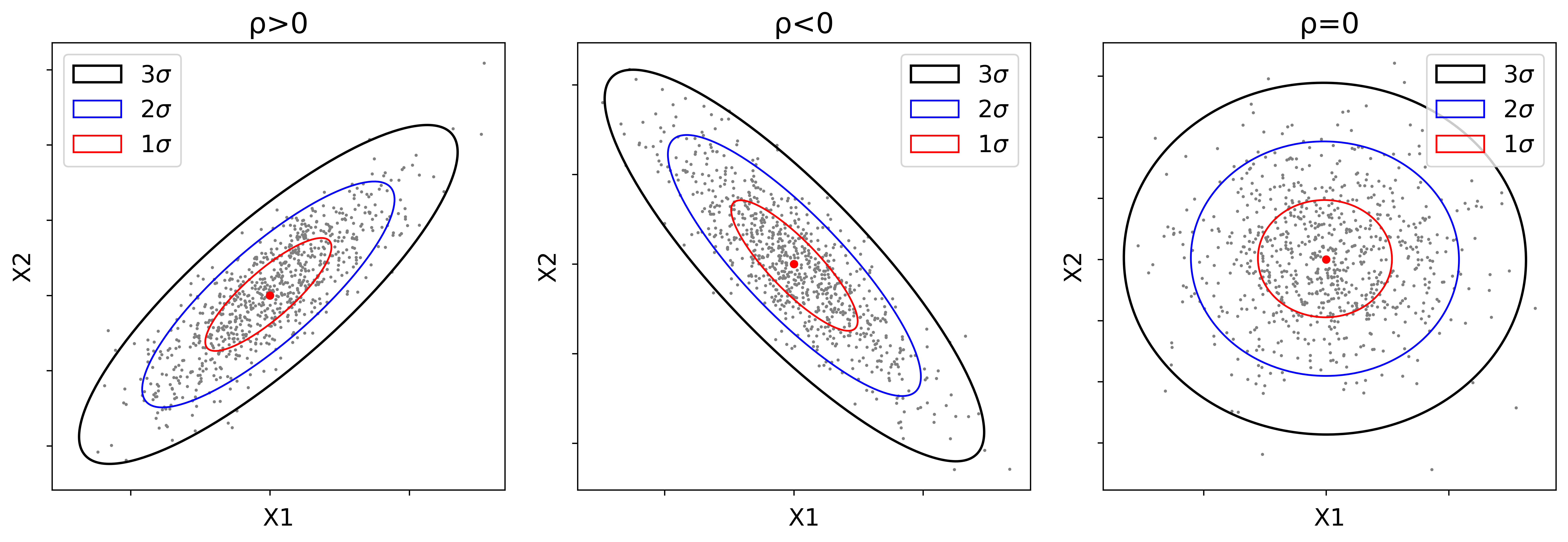
This figure shows how the ranges (or lengths) and directions of the axes of the ellipses change depending on the selected confidence level and the covariance matrix of the random vector \(\mathbf{X}\). The confidence ellipses constructed based on the given confidence levels can be used to check the bivariate Gaussianity of a given distribution (J. L. Deutsch & Deutsch, 2011).

Step 1: Selecting a probability level for the error ellipse

The quadratic form defining the scalar random variable \(K\) has a chi-square distribution \(\chi^{2}_{2}(\alpha)\) with two degrees of freedom:

\[P\left\{K\le \chi^{2}_{2}(\alpha)\right\} = P\left\{(\mathbf{X}-\boldsymbol {\mu})^{T}\Sigma^{-1}(\mathbf{X}-\boldsymbol{\mu})\le \chi^{2}_{2}(\alpha)\right\}=1-\alpha\]

where \(\chi^{2}_{2}(\alpha)\) is the upper \((100\alpha)th\) percentile of the \(\chi^{2}\)-distribution with two degrees of freedom. \(1-\alpha\) is the probability (or a confidence level) that the value of the random vector \(\mathbf{X}\) will be inside the ellipse. For example, consider that the given probability is \(\alpha=0.05\), that is, \(\chi^{2}_{2}(0.05)=5.99\), then the \(95\%\) confidence ellipse is defined by:

\[P\left\{K\le \chi^{2}_{2}(0.05)\right\} = P\left\{(\mathbf{X}-\boldsymbol {\mu})^{T}\Sigma^{-1}(\mathbf{X}-\boldsymbol{\mu})\le 5.99\right\}=0.95\]

Step 2: Calculating the eigenvalues of the covariance matrix

The positive definite (\(|\Sigma|\ne 0\) and \(\Sigma^{-1}\) exists) covariance matrix \(\Sigma\) of the random vector \(\mathbf{X} = [X_{1}, X_{2}]\) is as follows:

\[\Sigma= \begin{bmatrix} \sigma_{11} & \sigma_{12}\\ \sigma_{21} & \sigma_{22}\\ \end{bmatrix}\]

The eigenvalues \(\boldsymbol{\lambda}=[\lambda_{1}, \lambda_{2}]\) of \(\Sigma\) are calculated by:

\[ \lambda_{1}=\dfrac{1}{2}\left[\sigma_{11}+\sigma_{22}+\sqrt{(\sigma_{11}-\sigma_{22})^{2}+4\sigma_{11}\sigma_{22}\rho^{2}}\hspace{3pt}\right]\\\\ \lambda_{2}=\dfrac{1}{2}\left[\sigma_{11}+\sigma_{22}-\sqrt{(\sigma_{11}-\sigma_{22})^{2}+4\sigma_{11}\sigma_{22}\rho^{2}}\hspace{3pt}\right] \]

where \(\sigma_{11}\) and \(\sigma_{22}\) are the variances of the random variables \(X_{1}\) and \(X_{2}\), and \(\rho\) is the linear correlation coefficient.

Step 3: Calculating the lengths of the ellipse axes

The lengths of the ellipse axes are a function of the given probability \(\chi^{2}_{2}(\alpha)\), the eigenvalues \(\boldsymbol{\lambda}=[\lambda_{1}, \lambda_{2}]\) and the linear correlation coefficient \(\rho\). For example, \(95\%\) confidence ellipse is defined by:

\[[X_{1}-\mu_{1}\hspace{5pt}X_{2}-\mu_{2}]\hspace{3pt}\Sigma^{-1}\begin{bmatrix} X_{1}-\mu_{1}\\ X_{2}-\mu_{2}\\ \end{bmatrix} \le \chi^{2}_{2}(0.05) \]

As \(\Sigma\) denotes a symmetric matrix and \(\sigma_{11}\ne \sigma_{22}\), the eigenvectors of \(\Sigma\) is linearly independent (or orthogonal). Therefore, \(\Sigma\) can be written as follows:

\[\Sigma=TDT^{-1}\]

where \(T=[\upsilon_{1}|\upsilon_{2}]\) are the eigenvectors of \(\Sigma\) and \(D\) is the diagonal matrix of the eigenvalues \(\boldsymbol{\lambda}=[\lambda_{1}, \lambda_{2}]\):

\[D= \begin{bmatrix} \lambda_{1} & 0\\ 0 & \lambda_{2}\\ \end{bmatrix}\] replacing \(\Sigma^{-1}\) by \(TD^{-1}T^{-1}\), the square of the difference can be written as: \[[X_{1}-\mu_{1}\hspace{5pt}X_{2}-\mu_{2}]\hspace{3pt}TD^{-1}T^{-1}\begin{bmatrix} X_{1}-\mu_{1}\\ X_{2}-\mu_{2}\\ \end{bmatrix} \le \chi^{2}_{2}(0.05) \]

Denoting

\[\begin{bmatrix} \omega_{1}\\ \omega_{2}\\ \end{bmatrix} = T^{-1}\begin{bmatrix} X_{1}-\mu_{1}\\ X_{2}-\mu_{2}\\ \end{bmatrix} \]

As \(T^{T}=T^{-1}\), the square of difference can be expressed as:

\[[\omega_{1}\hspace{5pt}\omega_{2}]\hspace{3pt}\begin{bmatrix} \lambda_{1} & 0\\ 0 & \lambda_{2}\\ \end{bmatrix}^{-1}\hspace{3pt} \begin{bmatrix} \omega_{1}\\ \omega_{2}\\ \end{bmatrix} \le \chi^{2}_{2}(0.05) \]

If the above equation is further evaluated, The resulting equation is the equation of an ellipse aligned with the axis \(\omega_{1}\) and \(\omega_{2}\) in the new coordinate system.

\[\dfrac{\omega^{2}_{1}}{\chi^{2}_{2}(0.05)\lambda_{1}}+\dfrac{\omega^{2}_{2}}{\chi^{2}_{2}(0.05)\lambda_{2}}\le 1\]

The axes of the ellipse are defined by \(\omega_{1}\) axis with a length \(2\sqrt{\chi^{2}_{2}(0.05)\lambda_{1}}\) and \(\omega_{2}\) axis with a length \(2\sqrt{\chi^{2}_{2}(0.05)\lambda_{2}}\).

When \(\rho=0\), the eigenvalues are equal to \(\lambda_{1}=\sigma_{11}\) and \(\lambda_{2}=\sigma_{22}\). Also, \(T\) matrix whose elements are the eigenvectors of \(\Sigma\) becomes an identity matrix. The final equation of an ellipse is then defined by:

\[\dfrac{(X_{1}-\mu_{1})^{2}}{\chi^{2}_{2}(0.05)\lambda_{1}}+\dfrac{(X_{2}-\mu_{2})^{2}}{\chi^{2}_{2}(0.05)\lambda_{2}}\le 1\]

It is clear from the equation given above that the axes of the ellipse are parallel to the coordinate axes. The lengths of the axes of the ellipse are then defined as \(2\sqrt{\sigma_{11}\chi^{2}_{2}(0.05)}\) and \(2\sqrt{\sigma_{22}\chi^{2}_{2}(0.05)}\). Figure 2 displays \(95\%\) confidence ellipses drawn when the variables are positively correlated and when they are independent.

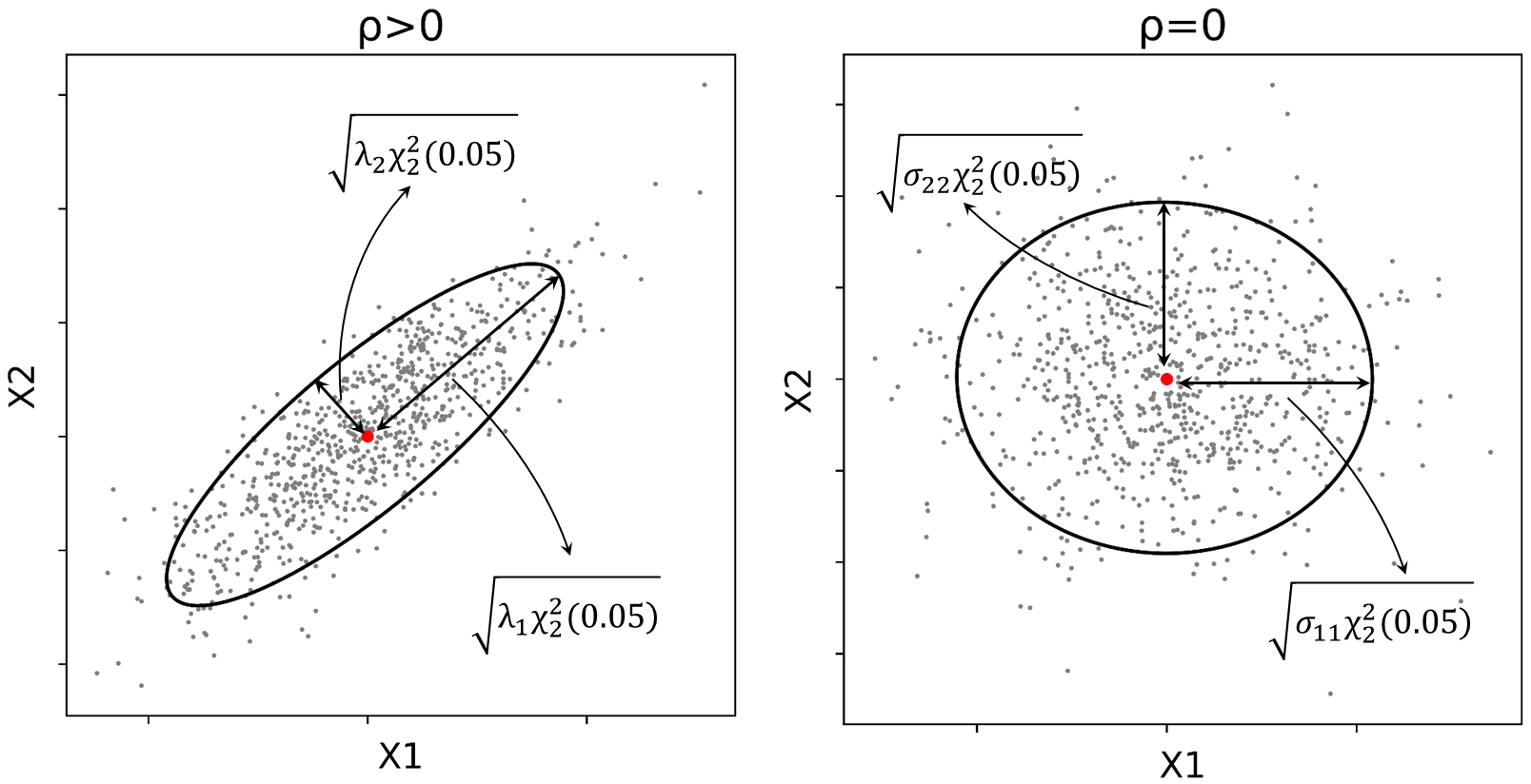
It is clearly seen from Figure 2 that when \(\rho>0\), the axes of the ellipse are aligned with the rotated axes in the transformed coordinate system, and when \(\rho=0\), axes of the ellipse are parallel to the original coordinate system.

Error Ellipses Method

The error ellipses method, first introduced by (Blachman, 1989), aims to combine individual probability distributions by the linear weighted averaging of the means. The optimal weighting minimizes the resulting variance of the combined distribution:

\[C_{\overline{\mathbf{x}}}=\left[\sum\limits_{i=1}^{n}C^{-1}_{i}\right]^{-1}\]

where \(C_{\overline{x}}\) is the minimized covariance matrix of the combined probability distribution, and \(C^{-1}_{i}\) is the covariance matrix of the individual probability distributions. The estimated mean vector of the combined distribution is then defined by:

\[\overline{\mathbf{x}}=C_{\overline{\mathbf{x}}}\left[\sum\limits_{i=1}^{n}C^{-1}_{i}\mathbf{x}_{i}\right]\]

where \(\overline{\mathbf{x}}\) is the mean of the combined probability distribution.

Derivation of the Error Ellipse Equations-1D Case

Consider that \(\{x_{i}; i=1,...,n\}\) are the means of \(n\) number of probability distributions, and \(\{\sigma^{2}_{i}; i=1,...,n\}\) are the corresponding variances of these probability distributions. The unbiased estimate of the mean of the combined probability distribution is defined by:

\[\overline{x}=\dfrac{\sum\limits_{i=1}^{n} \lambda_{i}x_{i}}{\sum\limits_{i=1}^{n}\lambda_{i}}\]

The variance of the estimate \(\overline{x}\) can be written as:

\[Var[\overline{x}] = \sum\limits_{i=1}^{n} \left[\lambda_{i} / \sum\limits_{i=1}^{n}\lambda_{i}\right]^{2} Var[\overline{x}_{i}]\]

Recall that \(Var[\overline{x}]=E[\overline{x}^{2}]-\{E[\overline{x}]\}^{2}\). Differentiating the equation given above with respect to \(\lambda_{j}\) guarantees the condition for the variance to be minimum:

\[\lambda_{j}Var[\overline{x}_{j}]=\dfrac{\sum\limits_{i=1}^{n}\lambda^{2}_{i}Var[\overline{x}_{i}]}{\sum\limits_{i=1}^{n}\lambda_{i}}\]

The right hand side of the equation does not depend on \(j\) and therefore, \(\lambda_{j}\) is proportional to \(1/Var[\overline{x} _{j}]\). Substituting these weights into the first and second equations given above yields:

\[\overline{x}=\left[\sum\limits_{i=1}^{n}Var[\overline{x}_{i}]^{-1}\right]^{-1} \sum\limits_{i=1}^{n}Var[\overline{x}_{i}]^{-1}\overline{x}_{i}\]

\[Var[\overline{x}]=\left[\sum\limits_{i=1}^{n}Var[\overline{x}_{i}]^{-1}\right]^{-1}\]

Finally, the mean of the combined distribution with the minimized variance can then be defined by:

\[\overline{x}=Var[\overline{x}]\sum\limits_{i=1}^{n}Var[\overline{x}_{i}]^{-1}\overline{x}_{i}\]

Derivation of the Error Ellipse Equations in a Multivariate Case

Consider \(m\) independent sets of observations, \(\textbf{O} =[O_{1},...,O_{m}]\) of the same target. Each observation \(O_{i}\), \(i=1,\ldots,m\) is an individual estimate of the target. The error ellipse of each observation is a contour of the Gaussian conditional probability density function \(P(x,y|O_{i})\) of the target (Blachman, 1989). Considering the Bayes’ theorem, for which the readers could refer to the lesson by (C. V. Deutsch & Deutsch, 2018), the aforementioned posterior distribution based on one set of observation can be defined by:

\[P(x,y|O_{i})=\dfrac{P_{i}(x,y)*P(O_{i}|x,y)}{P(O_{i})}\]

Provided that \(P_{i}(x,y)\) is constant over the area of interest, the posterior distribution can be defined by:

\[P(O_{i}|x,y)=\dfrac{P(O_{i})*P(x,y|O_{i})}{P_{i}(x,y)}\]

Assuming that each posterior distribution \(P(O_{i}|x,y)\) is independent, the total conditional probability over all observations, \(P(O_{1},\ldots,O_{m}|x,y)\) can then be defined as the product of individual posterior distributions \(P(O_{i}|x,y)\), that is,

\[P(O_{1},\ldots,O_{m}|x,y) =\prod_{i=1}^{m} \dfrac{P(O_{i})*P(x,y|O_{i})}{P_{i}(x,y)}\]

The conditional probability of the target given all observations is defined by the following function:

\[P(x,y|O_{1},\ldots,O_{m})=\dfrac{P(x,y)}{P(O_{1},\ldots,O_{m})}*\prod_{i=1}^{m} \dfrac{P(O_{i})*P(x,y|O_{i})}{P_{i}(x,y)}\]

Because the prior \(P(x,y)\) and \(P_{i}(x,y)\) are assumed to be constant over the area of interest, they cancel out. \(P(O_{i})\) and \(P(O_{1},\ldots,O_{m})\) depend only on the observation and are normalizing constants. Therefore, the conditional probability distribution of the target given all observations are defined as follows:

\[P(x,y|O_{1},\ldots,O_{m})=K*\prod_{i=1}^{m} P(x,y|O_{i})\]

Because \(P(x,y|O_{i})\) is Gaussian, its conditional probability density function can be defined by:

\[P(\mathbf{x}|\mathbf{O}_{1},\ldots,\textbf{O}_{m})=K*exp \left\{- \dfrac{1}{2}\sum\limits_{i=1}^{m}(\mathbf{x}-\mathbf{O} _{i})^{T}\mathbf{C}^{-1}_{i}(\mathbf{x}-\mathbf{O}_{i})\right\}\] where \(K\) is the scaling factor; \(\mathbf{x}\) is the vector defining target location; \(\mathbf{O}_{i}\) is the observation of \(\mathbf{x}\) and \(\mathbf{C}^{-1}_{i}\) is the covariance matrix of \(\mathbf{x}\). As with the 1-d case, the combined variance will be minimum which will be achieved by differentiating the probability density function given above:

\[\dfrac{\partial p}{\partial \textbf{x}}=K*e^{E_{m}}\left\{-\dfrac{1}{2}\dfrac{\partial E_{m}}{\partial \textbf{x}}\right\}\]

where \(E_{m}\) is defined by:

\[E_{m}=\sum\limits_{i=1}^{m}(\mathbf{x}-\mathbf{O}_{i})^{T}\mathbf{C}^{-1}_{i}(\mathbf{x}-\mathbf{O}_{i})\]

\[ \begin{split} \dfrac{\partial E_{m}}{\partial \textbf{x}}= \begin{bmatrix} \dfrac{\partial E_{m}}{\partial x_{1}}\\ \vdots \\ \dfrac{\partial E_{m}}{\partial x_{n}} \end{bmatrix} \end{split} \]

where \(m\) is the number of observations and \(n\) is the dimensionality of the vector \(\mathbf{x}\) and \(\mathbf{O}\). Consider the case where there is a single obervation, \(\textbf{O}_{1}\) then,

\[\begin{split} E_{1}&=(\mathbf{x}-\mathbf{O}_{1})^{T}\mathbf{C}^{-1}_{1}(\mathbf{x}-\mathbf{O}_{1})\\ &=\begin{bmatrix} x_{1}-O_{11}& \cdots & x_{n}-O_{1n}\\ \end{bmatrix}\begin{bmatrix} B_{11} & \cdots & B_{1n} \\ \vdots & & \vdots \\ B_{n1} & \cdots & B_{nn} \\ \end{bmatrix}\begin{bmatrix} x_{1}-O_{11}\\ \vdots\\ x_{n} - O_{1n}\\ \end{bmatrix}\\ &=\begin{bmatrix} \sum\limits_{i=1}^{n} B_{i1}(x_{i}-O_{1i})& \cdots & \sum\limits_{i=1}^{n} B_{in} (x_{i}-O_{1i})\\ \end{bmatrix}\begin{bmatrix} x_{1}-O_{11}\\ \vdots\\ x_{n} - O_{1n}\\ \end{bmatrix}\\ &=\sum\limits_{j=1}^{n}(x_{j}-O_{1j})\sum\limits_{i=1}^{n}B_{ij}(x_{i}-O_{1i}) \end{split} \]

Taking the derivative of the above equation with respect to \(x\)

\[\dfrac{\partial E_{1}}{\partial x_{k}} =\sum\limits_{i=1}^{n}B_{ik}(x_{i}-O_{1i})+\sum\limits_{j=1}^{n}B_{ki}(x_{j}-O_{1j})\]

Because the indices \(i\) and \(j\) both sum to one, the entire equation can be written as follows:

\[ \begin{split} \dfrac{\partial E_{1}}{\partial x_{k}} &=\sum\limits_{i=1}^{n}B_{ik}(x_{i}-O_{1i})+\sum\limits_{i=1}^{n}B_{ki}(x_{i}-O_{1i})\\ &=2\sum\limits_{i=1}^{n}B_{ki}(x_{i}-O_{1i})\\ &=2\mathbf{C}^{-1}_{1}(\mathbf{x}-\mathbf{O}_{1}) \end{split} \]

Setting the derivative to zero

\[ \begin{split} 2\mathbf{C}^{-1}_{1}(\mathbf{x}-\mathbf{O}_{1})&=0\\ \mathbf{C}^{-1}_{1}\mathbf{x}-\mathbf{C}^{-1}_{1}\mathbf{O}_{1}&=0\\ \mathbf{x}&=\mathbf{O}_{1} \end{split} \]

If only one set of observation \(\mathbf{O}_{i}\) is considered, the best estimation of the target’s location \(\mathbf{x}\) will be equal to that obervation \(\mathbf{O}_{i}\) (Orechovesky Jr, 1996). Expanding the estimation by considering \(m\) observations:

\[ \begin{split} E_{M}&=\sum\limits_{m=1}^{M}\left(\sum\limits_{j=1}^{n}(x_{j}-O_{mj})\sum\limits_{i=1}^{n}B_{ij}(x_{i}-O_{mi}\right)\\ &=\sum\limits_{m=1}^{M}(\mathbf{x}-\mathbf{O}_{m})^{T}\mathbf{C}^{-1}_{m}(\mathbf{x}-\mathbf{O}_{m})\\ \end{split} \]

Taking the derivative of the above equation with respect to \(\mathbf{x}\)

\[ \dfrac{\partial E_{n}}{\partial \textbf{x}} =2\sum\limits_{i=1}^{n}\textbf{C}^{-1}_{i}(\overline{\textbf{x}}-\textbf{O}_{i})\]

Setting the derivative to zero

\[ \begin{split} \sum\limits_{m=1}^{M}\left[\textbf{C}^{-1}_{i}(\overline{\mathbf{x}}-\mathbf{O}_{m})\right]&=0\\ \left(\sum\limits_{m=1}^{M}\textbf{C}^{-1}_{m}\right)\overline{\mathbf{x}}-\sum\limits_{m=1}^{M}(\mathbf{C}^{-1}_{m}\mathbf{O}_{m})&=0\\ \dfrac{1}{\left(\sum\limits_{m=1}^{M}\textbf{C}^{-1}_{m}\right)} \left(\sum\limits_{m=1}^{M}\textbf{C}^{-1}_{m}\right)\overline{\mathbf{x}}-\sum\limits_{m=1}^{M}(\mathbf{C}^{-1}_{m}\mathbf{O}_{m})\dfrac{1}{\left(\sum\limits_{m=1}^{M}\textbf{C}^{-1}_{m}\right)}&=0\\ \overline{\mathbf{x}}-\sum\limits_{m=1}^{M}\mathbf{C}(\textbf{C}^{-1}_{m}\mathbf{O}_{m})&=0 \end{split} \]

Finally, the combined mean \(\overline{\mathbf{x}}\) and variance \(\mathbf{C}\) are defined by:

\[\overline{\mathbf{x}}=\mathbf{C}\sum\limits_{m=1}^{M}\left(\mathbf{C}^{-1}_{m}\mathbf{O}_{m}\right), \hspace{4pt}\hspace{4pt}\mathbf{C}=\left(\sum\limits_{m=1}^{M}\mathbf{C}^{-1}_{m}\right)^{-1}\]

Example

Consider two bivariate Gaussian distributions, \(\mathbf{X}, \mathbf{Y} \sim N(\boldsymbol{\mu},\Sigma)\). The variables of these random vectors are \(\mathbf{X} = [X_{1},X_{2}]\) and \(\mathbf{Y} = [Y_{1},Y_{2}]\). The parameters of the aforementioned bivariate Gaussian distributions are \(\boldsymbol{\mu}_{X}=[4, 6]\), \(\boldsymbol{\mu}_{Y}=[3,8]\) and \((2\times 2)\) positive definite covariance matrices \(\Sigma_{\mathbf{X}}\), \(\Sigma_{\mathbf{Y}}\) are:

\[\Sigma_{\mathbf{X}} = \begin{bmatrix} 0.7 & 0.9\\ 0.9 & 1.9\\ \end{bmatrix} \hspace{4pt} \hspace{4pt} \Sigma_{\mathbf{Y}} = \begin{bmatrix} 0.5& 0\\ 0 & 1.2\\ \end{bmatrix}\]

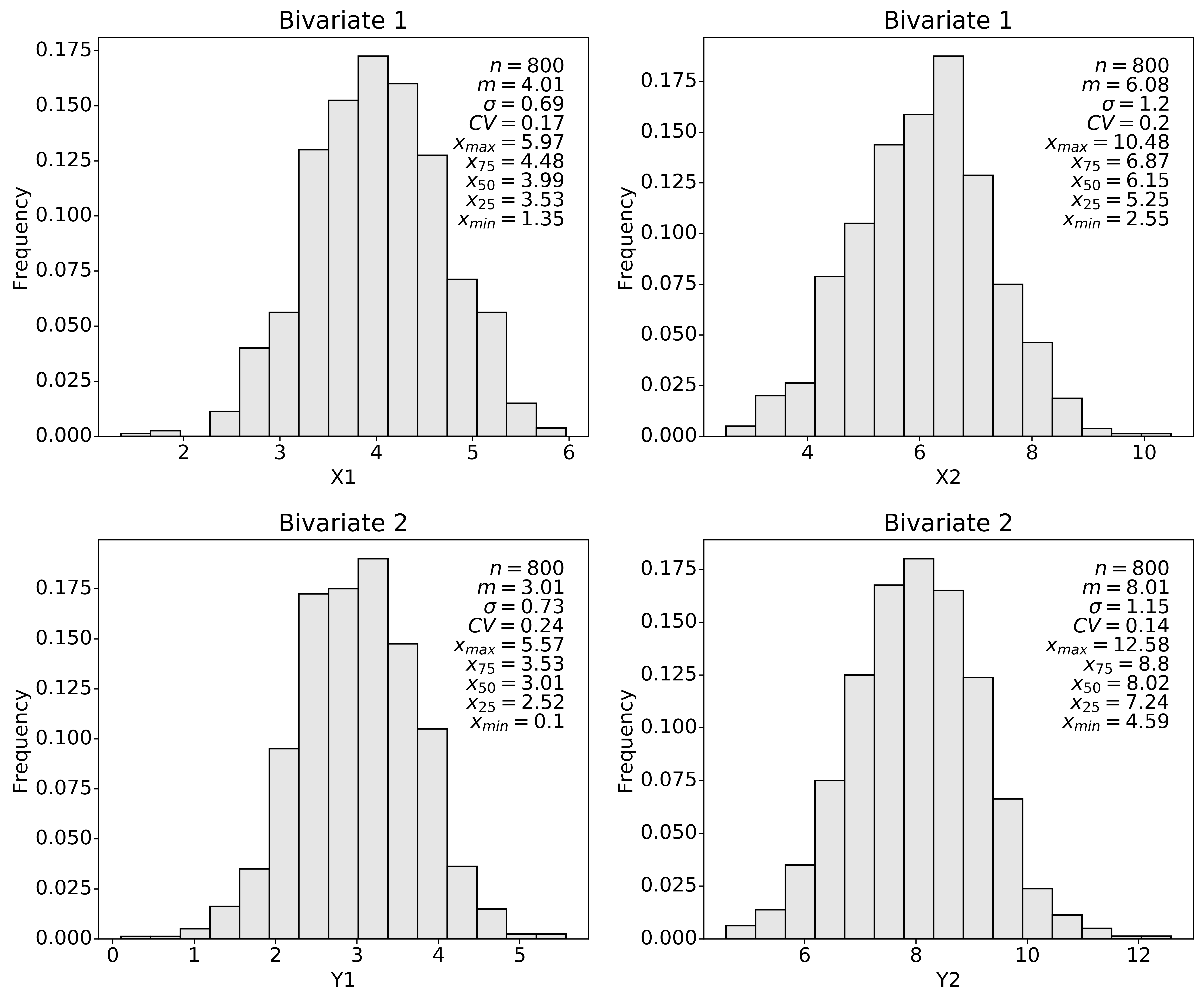
Based on the parameters given above, the variables, \(X_{1},X_{2}\) and \(Y_{1},Y_{2}\) were simulated. Let \(\{x^{k}_{1}, x^{l}_{2};\hspace{3pt} k,l=1,...,800\}\) be the simulated samples of \(X_{1},X_{2}\), and \(\{y^{k}_{1}, y^{l}_{2};\hspace{3pt}k,l=1,...,800\}\) be the simulated samples of \(Y_{1},Y_{2}\). The histograms of the samples of the simulated variables are given in Figure 3.

The probability level \((1-0.05 = 0.95)\), \(\chi^{2}_{2}(0.05)=5.99\) is first selected, as explained in Step 1. This means that \(95\%\) probability that the values of the random vectors \(\mathbf{X}\) and \(\mathbf{Y}\) will be inside the ellipses. The eigenvalues (Step 2) of \(\Sigma_{\mathbf{X}}\) and \(\Sigma_{\mathbf{Y}}\) are calculated to be \(\boldsymbol{\lambda}_{X}=[2.38, 0.22]\) and \(\boldsymbol{\lambda}_{Y} =[1.2, 0.5]\), respectively.

Considering the first bivariate Gaussian distribution defined by the random vector \(\mathbf{X}\), the variables are positively correlated \(\rho=0.78\). Therefore, the axes of the ellipse will point in the directions of the eigenvectors (Step 3). The eigenvectors of \(\Sigma_{\mathbf{X}}\) are calculated to be \(\mathbf{\upsilon_{1}} =[0.88, 0.47]^{T}\) and \(\mathbf{\upsilon_{2}}=[0.47, -0.88]^{T}\). The lengths of the ellipse axes are calculated to be \((2\sqrt{5.99\cdot 2.38}=7.55)\), \((2\sqrt{5.99\cdot 0.22}=2.3)\). The axes of the \(95\%\) confidence ellipse of the random vector \(\mathbf{X}\) are then defined by \(\pm\sqrt{5.99\cdot 2.38}\cdot [0.88, 0.47]^{T}\) and \(\pm \sqrt{5.99\cdot 0.22}\cdot [0.47, -0.88]^{T}\).

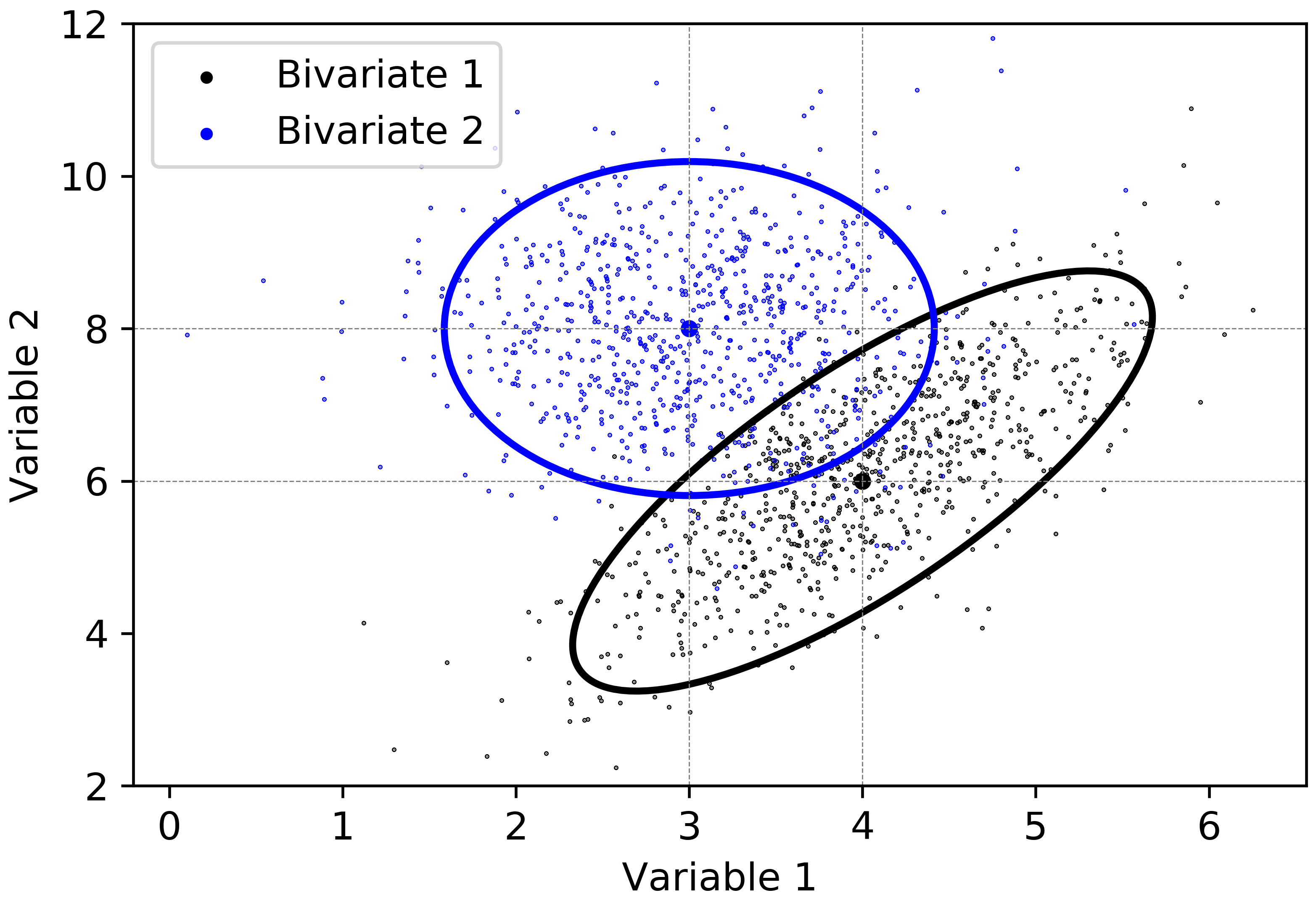
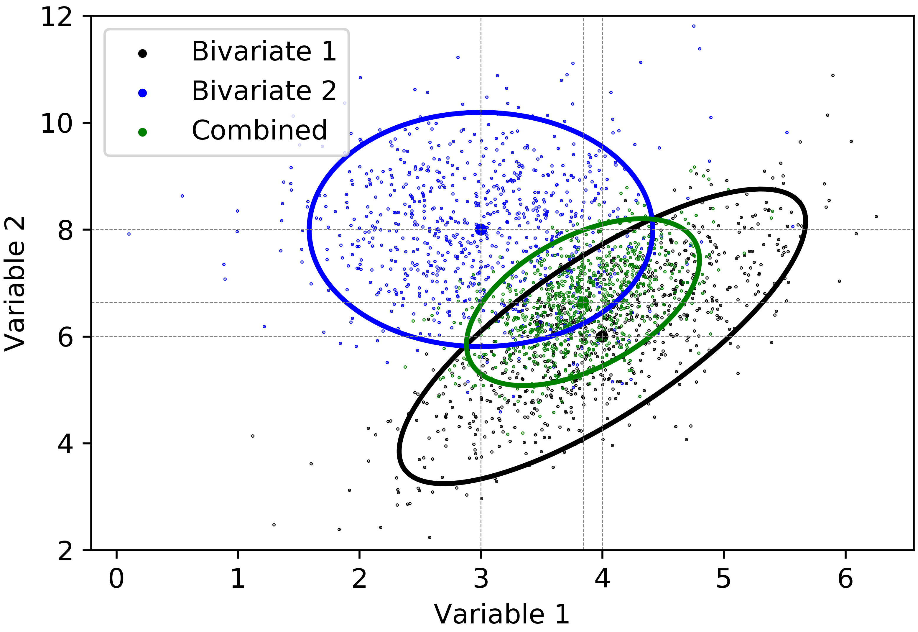
Considering the second bivariate Gaussian distribution defined by the random vector \(\mathbf{Y}\), the variables are independent. The eigenvalues of \(\Sigma_{\mathbf{Y}}\) are equal to the variances of \(Y_{1}\) and \(Y_{2}\), respectively. As explained in Step 3, the axes of the ellipse are parallel to the original coordinate axes. The lengths of the axes are calculated to be \((2\sqrt{5.99\cdot 1.2} =5.36)\), \((2\sqrt{5.99\cdot 0.5}=3.46\). The axes of the \(95\%\) confidence ellipse of the random vector \(\mathbf{Y}\) are then defined by \(\pm\sqrt{5.99\cdot 1.2}\cdot [0, 1]^{T}\) and \(\pm\sqrt{5.99\cdot 0.5}\cdot [1, 0]^{T}\). The \(95\%\) confidence ellipses for the given bivariate Gaussian distributions are displayed in Figure 4.

The variance \(C_{\overline{\mathbf{x}}}\) of the combined probability distribution is calculated as follows:

\[\begin{split} C_{\overline{\mathbf{x}}}&=\left(\begin{bmatrix} 0.7& 0.9\\ 0.9 & 1.9\\ \end{bmatrix}^{-1}+\begin{bmatrix} 0.5& 0\\ 0 & 1.2\\ \end{bmatrix}^{-1}\right)^{-1}\\ C_{\overline{\mathbf{x}}}&=\begin{bmatrix} 0.23& 0.19\\ 0.19 & 0.61\\ \end{bmatrix} \end{split}\]

and the mean vector of the combined distribution \(\overline{\mathbf{x}}\) is then defined by:

\[\begin{split} \overline{\mathbf{x}}&=\begin{bmatrix} 0.23& 0.19\\ 0.19 & 0.61\\ \end{bmatrix}\left(\begin{bmatrix} 0.7& 0.9\\ 0.9 & 1.9\\ \end{bmatrix}^{-1} \begin{bmatrix} 4 \\ 6 \\ \end{bmatrix}+\begin{bmatrix} 0.5& 0\\ 0 & 1.2\\ \end{bmatrix}^{-1} \begin{bmatrix} 3 \\ 8 \\ \end{bmatrix}\right)\\ \overline{\mathbf{x}}& = \begin{bmatrix} 3.84 \\ 6.64 \\ \end{bmatrix} \end{split}\]

Based on the estimated variance \(C_{\overline{\mathbf{x}}}\) and the mean \(\overline{\mathbf{x}}\), the bivariate Gaussian variables are simulated. \(95\%\) confidence ellipse of the combined distribution is given in Figure 5.

Summary

The error ellipses method combines probability distributions by a linear combination. The combined probability distribution is a convex estimation of the mean of the combined distribution, that is, the estimated mean of the combined distribution always falls between the means of the input probability distributions; the lower variance distribution has the greatest influence. This method is especially useful when there is no clear prior distribution, for example, in the estimation of parameters from diverse data sources. The method should not be used for spatial prediction when a reasonable prior model is available.

References