Learning Objectives

• Understand the nature of categorical variables in a geostatistical context
• Review parametric and non-parametric categorical variable distributions
• Assess the transition from categorical to continuous variables

Introduction

A continuous variable takes an outcome between some minimum and maximum. A categorical or discrete variable will take an outcome from a list of possible values. Categorical variables are often descriptive of some dominant geological characteristic; the outcomes could be thought of as labels with no intrinsic numerical meaning. The number of possible outcomes could be indexed, \(k=1,\ldots,K\), where there are typically less than seven, that is, \(K\leq 7\) (Deutsch, 2021). Examples of categorical variables could be rock types, facies, alteration, or mineralization types (Deutsch & Lan, 2008; Rossi & Deutsch, 2013).

The nature of categorical random variables is discussed. As scale increases, categories are mixed and the correct representation becomes a continuous proportion. Inference of the probability distributions and summary statistics for categorical variables are reviewed. This Lesson does not get into the importance of categorical variables in Geostatistics or the details of categorical variable modeling techniques; these subjects are important, but this Lesson provides an initial overview of categorical variable distributions.

Categorical Variables

Categorical variables are divided into ordinal, nominal, and interval. Each of these can be either dichotomous (binary), or polychotomous (multi‐category) (Silva, 2018). Ordinal variables have a natural ordering in the categories (e.g., degree of rock alteration). Nominal variables have no intrinsic ordering of the categories (e.g., lithology). Interval variables are ordered and the distance between the categories is known (e.g., classes of porosity) (Silva, 2018). In practice, interval categories are defined by a set of thresholds selected from a continuous variable. When possible, the categories should be sorted to improve modeling results (Deutsch, 2021). Often categorical variables are a nominal description or an indicator of a stationary domain.

Stationary Domains

A prerequisite when constructing numerical models is a conceptual geological model and a choice of reasonable subsets of the (1) data, and (2) unsampled volume. These subsets are often called stationary domains. These subsets may be defined hierarchically. Large scale limits may be defined deterministically and small scale domains may be defined by categorical variable modeling within the defined limits. The final domains should define geometric zones that are reasonably statistically homogeneous. The greatest variability should be between the domains and not within the domains. Categorical variable modeling typically precedes continuous variable modeling. Then, the continuous variables are modeled within each category.

The domains may be based on one or more intrinsic geologic characteristics such as facies, alteration, or mineralization types; however, they may be based on an underlying continuous variable with the purpose of isolating high and low values for improved prediction. The use of domains based on an underlying continuous variable is reasonable if the results are spatially coherent and predictable. In some cases, multiple categorical variables are modeled (e.g., mineralization types and alteration types) and final domains are based on a combination of the different categorical variables. Each situation is unique and depends on the relative importance of the different geological controls, the data spacing, the scale of variability among other factors. An extensive discussion of stationary domains can be found in a preceding Lesson (Dias & Deutsch, 2022) at GeostatisticsLessons.com.

Categorical Variables Statistics

The \(K\) outcomes of a categorical variable \(Z\) are mutually exclusive and exhaustive (Derakhshan & Deutsch, 2009a; Rossi & Deutsch, 2013). Every location \(\mathbf{u}_j, j=1,\ldots,n\), belongs to one category, and there is no intersection, overlap, or gap between them. Indicators are adopted to lend numerical meaning to categorical variables and perform statistics. Analytically, \(i(\mathbf{u} ; k)\) denotes an indicator variable corresponding to category \(k\), considering a location \(\mathbf{u}\). If \(\mathbf{u}\) belongs to \(k\), the indicator is 1; otherwise, it is 0 (Rossi & Deutsch, 2013). The number of indicators equals \(K\). Therefore, our \(z(\mathbf{u}_j), j=1,\ldots,n\), sampled data become \(K\) sets of \(n\) indicator data.

\[ i(\mathbf{u}_j ; k)=\left\{\begin{array}{ll} 1, & \text { if location } \mathbf{u}_j \text { belongs to } k \\ 0, & \text { otherwise } \end{array}, \quad j=1, \ldots, n, \quad k=1, \ldots, K\right. \] The term \(j\) denotes the number of locations, \(j=1,\ldots,n\), and \(k\) the number of categories \(k=1,\ldots,K\).

The probability or proportion \(p_k\) of \(k\) is calculated by the mean indicator corresponding to \(k\). The probability distribution is defined by the probability of each category (Pyrcz & Deutsch, 2014). In practice, sample bias is considered; consequently, the proportions, \(p_k, k=1,\ldots,K\), are calculated considering declustering weights \((w_j, j=1,\ldots,n)\) (Rossi & Deutsch, 2013):

\[ p_k=\frac{\sum_{j=1}^n w_j i\left(\mathbf{u}_j ; k\right)}{\sum_{j=1}^n w_j}, \quad k=1, \ldots, K \]

There are three common methods of declustering; cell, polygonal, and estimation weight declustering (Deutsch & Deutsch, 2015; Pyrcz & Deutsch, 2002).

The variance of the indicator variable of \(k\) can be calculated (Rossi & Deutsch, 2013):

\[ \operatorname{Var}\left\{i\left(\mathbf{u} ; k\right)\right\}=\frac{\sum_{j=1}^n w_j\left[i\left(\mathbf{u}_j ; k\right)-p_k\right]^2}{\sum_{j=1}^n w_j}=p_k\left(1-p_k\right), \quad k=1, \ldots, K \] Indicator variances are useful in variogram standardization, facilitating interpretation and comparison among categories.

Non Parametric Categorical Variables Distributions

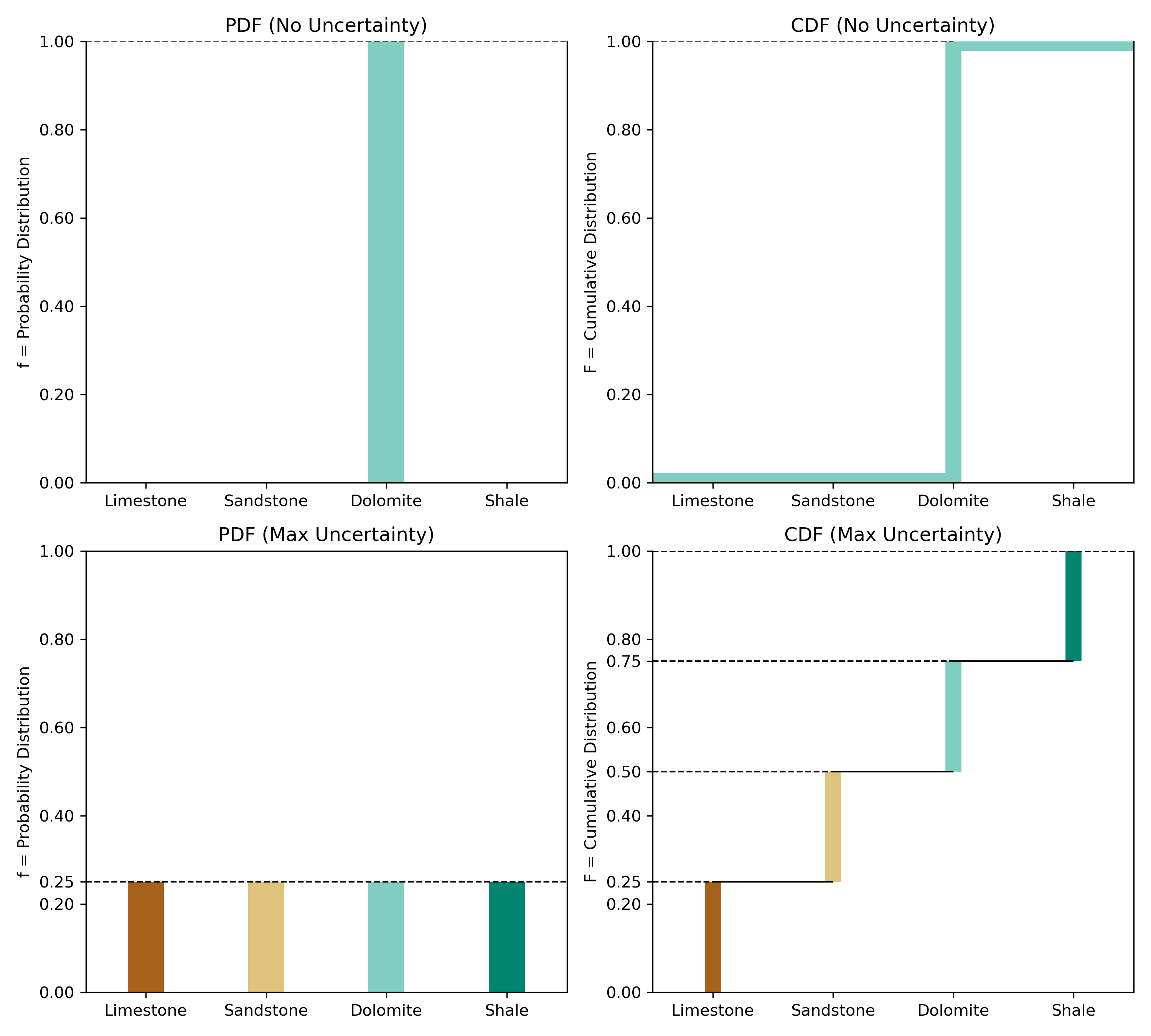
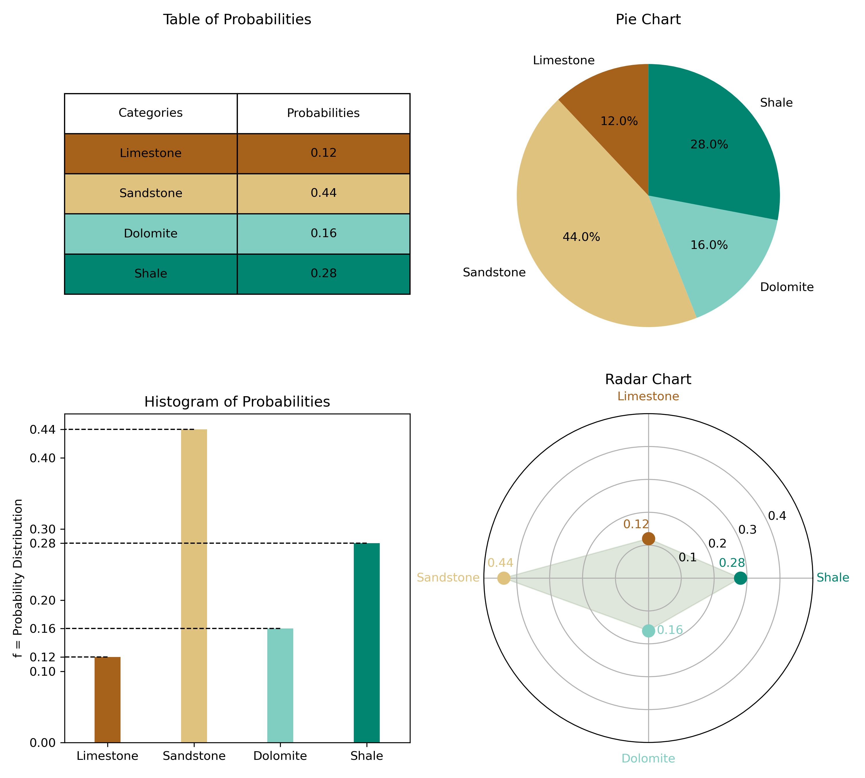
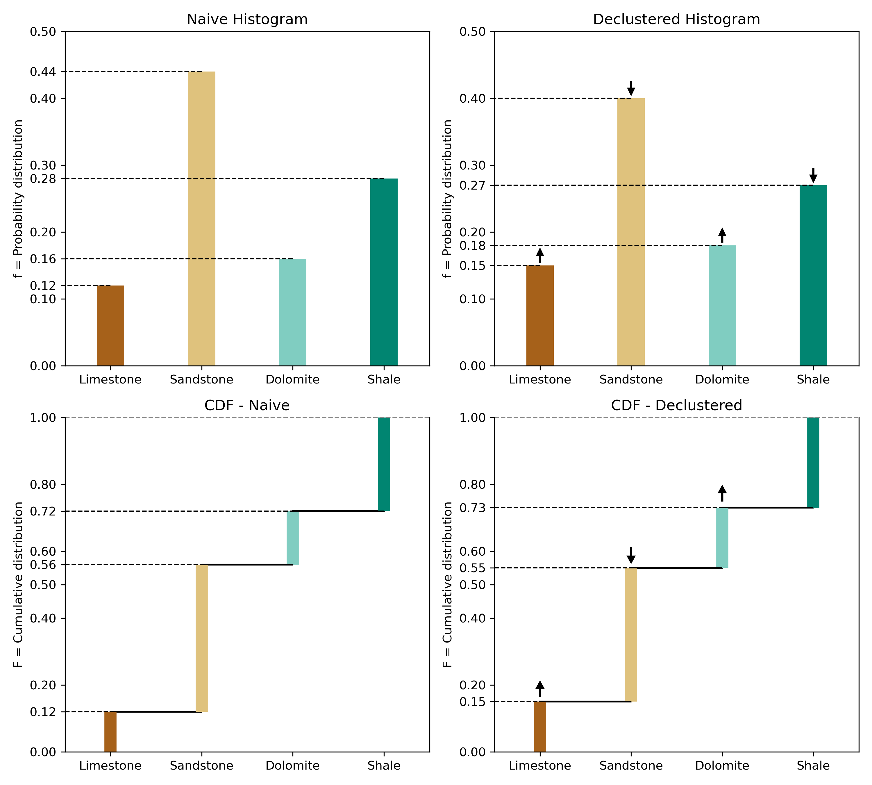
The sum of the \(p_k\) proportions must be equal to 1, that is, \(\sum_{k=1}^K p_k=1\), and none of them can be negative, \(p_k \geq 0, k=1,\ldots, K\) (Pyrcz & Deutsch, 2014). Perfect knowledge is when one \(p_k=1\), and all other \(p_{k^{\prime}}\) values are 0, \(k^{\prime} \neq k\). Complete uncertainty is \(p_k=1 / K\) for all categories (a uniform distribution) (Deutsch, 2021). Figure 1 illustrates the PDF and CDF of both cases. Generally, global proportions inform us that some categories are more probable (Deutsch, 2021). The global or prior proportions inferred from declustering are used for exploratory data analysis and local inference. A probability density function (PDF) of a categorical variable can be fully represented by a table of probabilities, a pie chart, a histogram of probabilities, or a radar chart (Figure 2). The cumulative distribution function (CDF) is represented as well, taking the actual categories and arbitrarily ordering them in a series of step functions. The CDF is useful in Monte Carlo simulation and data transformation. An example of a typical categorical PDF and CDF is given in Figure 3, along with their declustered representations (Pyrcz & Deutsch, 2014; Rossi & Deutsch, 2013).

Univariate Probability Density Function

Once the random categorical variable \(Z(\mathbf{u})\) has been defined, a PDF is defined as well, and expressed as:

\[ f\left(\mathbf{u} ; k\right)=\operatorname{Prob}\left\{Z(\mathbf{u}) \in k\right\}, \quad k=1, \ldots, K \] where, \(f(\mathbf{u} ; k) \geq 0\), and \(\sum f(\mathbf{u} ; k)=1\). The notation \(f(k)\) is used instead of \(p_k\) to maintain consistency with the multivariate representation below.

The univariate PDF gives the set of probabilities \(\left\{p_1, \dots, p_K\right\}\) associated with each of the categories that can be observed in an unsampled location \(\mathbf{u}\) (Li, 2011). Consider the declustered PDF in Figure 3; sandstone is the most probable.

Bivariate and Multivariate Probability Density Function

The univariate PDF is useful in characterizing the uncertainty at an unsampled location. Nevertheless, the uncertainty regarding either two, or more locations together is of interest. The bivariate and multivariate PDFs for a categorical variable \(Z(\mathbf{u}_1,\mathbf{u}_2)\) and \(Z(\mathbf{u}_1, \ldots, \mathbf{u}_n)\), respectively, are defined as:

\[ f\left(\mathbf{u}_1, \mathbf{u}_2 ; k_1, k_2\right)=\operatorname{Prob}\left\{Z\left(\mathbf{u}_1\right) \in k_1, Z\left(\mathbf{u}_2\right) \in k_2\right\}, \quad k_1, k_2=1,\ldots,K \] and,

\[ f\left(\mathbf{u}_1, \ldots, \mathbf{u}_n ; k_1,\ldots, k_n\right)=\operatorname{Prob}\left\{Z\left(\mathbf{u}_1\right) \in k_1, \ldots, Z\left(\mathbf{u}_n\right) \in k_n\right\}, \quad k_1,\ldots,k_n=1,\ldots,K. \]

These determine the probability of joint outcomes either for two locations (bivariate), or for a group of \(n\) locations (multivariate). Once the multivariate PDF is established, all of the marginal ones can be obtained. The bivariate and multivariate PDFs entail the following conditions respectively: \(\sum f\left(\mathbf{u}_1, \mathbf{u}_2\right)=1\), and \(f\left(\mathbf{u}_1, \mathbf{u}_2\right) \geq 0\) (bivariate), \(\sum f\left(\mathbf{u}_1, \ldots, \mathbf{u}_n\right)=1\), and \(f\left(\mathbf{u}_1, \ldots, \mathbf{u}_n\right) \geq 0\) (multivariate) (Li, 2011; Pyrcz & Deutsch, 2014).

Entropy

The summary statistics derived from a univariate categorical PDF are mainly the proportions. Computing the variance \(\left(p_k\left(1-p_k\right)\right)\) does not provide any additional information. Nevertheless, we can quantify the uncertainty in the PDF, by the measure of entropy. For a categorical variable with \(K\) categories \(p_k, k=1,\ldots, K\), entropy can be calculated (Gray, 2011):

\[ H=-\sum_{k=1}^{K} p_k \ln \left(p_k\right) \]

When the variable is uniformly distributed, the entropy achieves its maximum value, corresponding to the least informative prediction (Li & Deutsch, 2009). In the opposite scenario, where there is sufficient information to identify the true category, \(p_k=1\), the entropy is zero (Sadeghi, 2017). Consider a categorical random variable \(Z\), where all possible categories (\(k, k=1,\ldots, K\)) are equally probable, \(p_k=1 / K\), the entropy then would be (Li & Deutsch, 2009):

\[ H_{\max }=-\sum_{k=1}^{K} \frac{1}{~K} \ln \left(\frac{1}{~K}\right)=-\ln \left(\frac{1}{~K}\right)=\ln K \]

Considering uniform probabilities, \(\ln K\) is the upper bound for the entropy with the least informative prediction (Li & Deutsch, 2009).

Transition from Categorical to Continuous Distributions

When larger volumes are considered, the categories are unavoidably mixed, forfeiting their mutual exclusivity and exhaustiveness. When the volume is increased, the indicator variable corresponding to \(k\) does not assume only 0 and 1; instead, a proportion of values between 0 and 1, is now considered (Deutsch & Lan, 2008). First, a neighborhood \(\mathrm{v}_j\) of locations \(\mathbf{u}_j, j=1, \ldots,n\), is defined, representing a specific volume – referred to as a “block” in Geostatistics. Consider \(m\) blocks at \(\mathrm{v}_j\) support. The proportion \(p_k\) of \(k\) in one block can be calculated (Derakhshan & Deutsch, 2009b; Deutsch & Lan, 2008; Lan, 2007):

\[ p_{k,\mathrm{v}}=\frac{1}{\mathrm{v}} \int_\mathrm{v} i\left(\mathbf{u}_{j_\mathrm{v}}, k\right) d\mathrm{v}, \quad k=1, \ldots,K \]

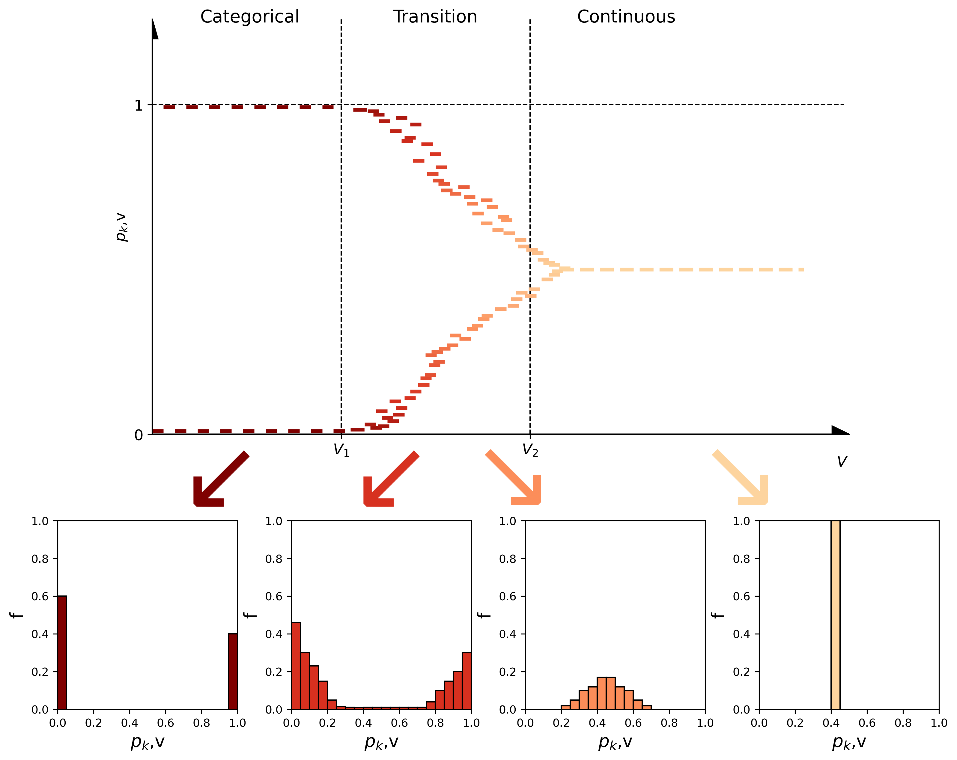
Assume that in one block, there are 8 points. The \(p_k\) of \(k\) in that block can take values from the set of \(\left\{0, \frac{1}{8}, \frac{2}{8}, \frac{3}{8}, \frac{4}{8}, \frac{5}{8}, \frac{6}{8}, \frac{7}{8}, 1\right\}\). The \(p_k\) values derive from each block define the distribution of the indicator variable corresponding to \(k\) at that specific scale \(\mathrm{v}_j\). In a scale \(\mathrm{v}\), \(p_k\) at each block can take values from the set \(\left\{0, \frac{1}{\mathrm{v}}, \frac{2}{\mathrm{v}}, \ldots, 1\right\}\). The larger the \(\mathrm{v}\), the larger the set. The univariate distribution for each indicator variable gradually changes from a bimodal distribution of ones and zeros, at the point scale, to unimodal at the global mean as the support increases (Derakhshan & Deutsch, 2009b; Lan, 2007).

At scale \(V_1\) the bimodal distribution becomes continuous between zero and one. \(V_1\) is called representative facies volume (RFV) (Derakhshan & Deutsch, 2009a). RFV stems from the notion of the representative elementary volume (REV). Figure 4 illustrates the concept of the transition from categorical to continuous distributions. An RFV plot has three regions (1) little or no mixing (categorical), (2) higher levels of mixing (transition), and (3) complete mixing (continuous). \(V_2\) is the scale where one block equals the size of the domain, therefore, the global proportions of the \(K\) categories prevail (Derakhshan & Deutsch, 2009a).

The CDFs of the two extreme cases at \(V=0\) and at \(V=\infty\) are illustrated in Figure 5. At the point scale, \(p_k\) takes either 0 or 1, at the largest scale \(p_k\) is the global proportion of the category \(k\) (Derakhshan & Deutsch, 2009b; Deutsch & Lan, 2008).

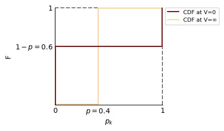
The mean of the scaled-up proportion remains unaffected by increasing the support. Assuming a uniform division of the entire space of interest into \(m\) equally-sized blocks, the mean of the proportion \(p_{k, \mathrm{v}}\) can be determined (Lan, 2007):

\[ E\left[p_{k, \mathrm{v}}\right]=\frac{1}{m} \frac{1}{n} \sum_{a=1}^m \sum_{j=1}^n i\left(\mathbf{u}_{j, a}, k\right), \quad k=1, \ldots, K \] where \(\mathbf{u}_j\), \(j=1,\ldots n\), represents the number of points within each of the \(m\) blocks.

On the other hand, the variance of the scaled-up proportion is reduced as the scale increases (Deutsch & Lan, 2008; Lan, 2007). The variance is scale-dependent. This lies in the concept of additivity of variance. Assuming that we consider three different scales: points \((\mathrm{v})\), blocks \((V)\), and the domain \((A)\). Then, the variance of point scale values in the domain \((D^2(\mathrm{v}, A))\) is equal to the variance of point scale values in the blocks \((D^2(\mathrm{v}, V))\) plus the variance of block scale values in the domain \((D^2(V, A))\) (Harding & Deutsch, 2019):

\[ D^2(\mathrm{v}, A)=D^2(\mathrm{v}, V)+D^2(V, A) \]

The topic of the additivity of variance is extensively covered in a previous Lesson (Harding & Deutsch, 2019) and can be found at GeostatisticsLessons.com.

Overall, beyond the RFV scale, any indicator simulation technique that assumes mutual exclusivity does not work well, hence determining the RFV is crucial to adopt the most appropriate modeling strategy (Derakhshan & Deutsch, 2009a; Razavi, 2013). Many categorical variables are somewhat subjective and logged by a geologist based on visual inspection. This logging is based on a chosen scale from the start, for example, it could be logged at a centimeter or a meter scale. In most cases, the scale of logging is related to the anticipated scale of geostatistical modeling.

Sum to Unity Constraint

The sum of the proportions \(\left(p_1, p_2, \ldots, p_K \geq 0\right)\) of a categorical variable must equal 1 at any scale considered for the distribution to be valid. This entails the following equation being satisfied at any \(V\) (Derakhshan & Deutsch, 2009b; Lan, 2007):

\[ p_1+p_2+\ldots+p_K=1 \]

Given that the sum of \(K\) proportions, \(p_1, p_2, \ldots, p_K\), equals one, plotting each proportion in \(K\)-dimensional space, will lead to a point that falls on a hyperplane (or a \(K-1\)-simplex). In the case of two categories, \(p_1\) and \(p_2\), the point must fall on a unit 1-simplex, which is a line segment connecting the vertices (1,0) and (0,1), satisfying the unity constraint and validating the distribution. Regarding three categories, \(p_1\), \(p_2\), and \(p_3\), in order for the distribution to be realistic, the point must lie on a unit 2-simplex, that is an equilateral triangle plane attaching the vertices (1,0,0), (0,1,0), and (0,0,1) (Derakhshan & Deutsch, 2009b; Lan, 2007). These statements regarding both cases are represented schematically in Figure 6.

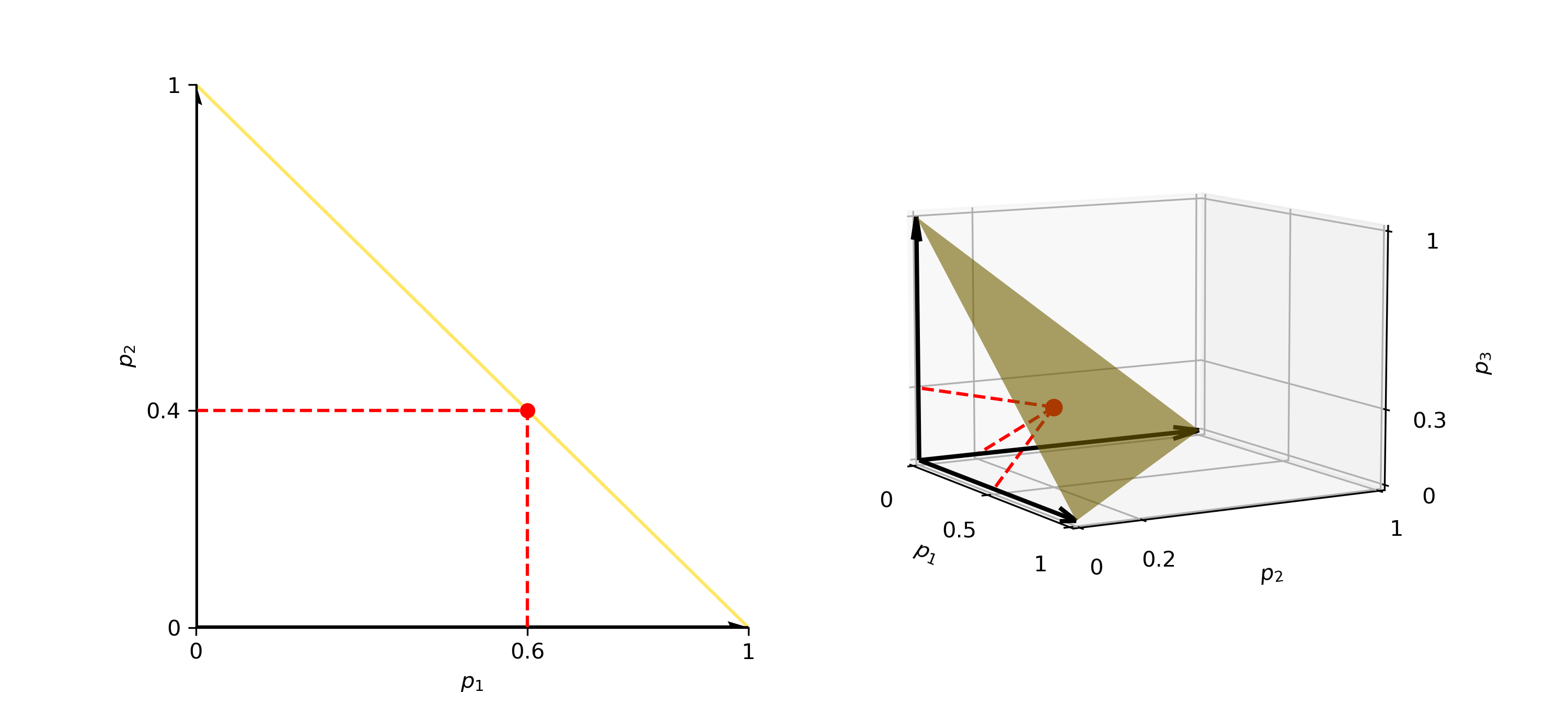
The sum to unity constraint requires the proportions of the categories to sum to 1, ensuring a physically meaningful and valid distribution at any scale. A simplex is a geometric shape representing this constraint in \(n\)-dimensional space. The \(K\)−1 simplex can be mathematically expressed (Derakhshan & Deutsch, 2009b):

\[ \Delta^{K-1}=\left\{\left(p_1, \ldots, p_K\right) \in R^K \mid \sum_{k=1}^K p_k=1 \text { and } p_k \geq 0 \text { for all } k\right\} \]

The resulting proportions must satisfy the unity constraint by lying on the surface of the simplex, making it an important consideration in categorical variables modeling.

Parametric Categorical Variable Distributions

Non-parametric categorical variable distributions are those derived directly from the data. For categorical variable distributions, we use non-parametric and, usually, non-stationary distributions. Although, sometimes we consider parametric categorical variable distributions, such as Beta distributions, the Binomial distribution, and Benford’s Law (Deutsch, 2021). These have rare applications in Geostatistics. Nevertheless, they are worth mentioning.

Beta Distributions

A category’s marginal probability distribution is changed when the volume is increased from discrete to continuous. The same is applied to the multivariate probability of the full set of categories as well. The continuous character of both distributions at higher supports depends on the means and variances of all categories. Therefore, fitting the data, based on the known means and variances is possible. The Beta distribution can be used in producing simulated realizations of each category’s marginal distribution at different supports. Dirichlet and Ordinary Beta distributions are useful for modeling the multivariate probability distribution of the categories at varying support, with the latter being considered more suitable (Deutsch & Lan, 2008; Lan, 2007).

Binomial Distribution

The Binomial distribution is a parametric categorical variable distribution applied in mining (Kennedy & Kennedy, 1990). It is useful in the presence of two mutually exclusive outcomes, calculating the probability of \(k\) successes, \(p_k\), out of \(n\) independent trials, where \(p\) is the probability of success of one trial (Agresti, 2012):

\[ p_k=\left(\begin{array}{l} n \\ k \end{array}\right) p^k(1-p)^{n-k}=\frac{n !}{k !(n-k) !} p^k(1-p)^{n-k}, \quad k=1, \ldots, K \]

As an example, non-continuous haulage systems in mining involve shovels operating within the mine site. The production rate of a fleet of shovels, \(R_f\), comprising \(n\) identical shovels, each with a production rate of \(r\), can be calculated:

\[ R_f=n r \]

Assuming the fleet’s production rate aligns with the required rate for plant feeding, the above equation could be applied to determine the necessary shovel count. This calculation assumes ideal coordination among operational shovels and constant availability of all. However, in practice, this is rarely the case as the availability of shovels is limited. Given the known availability, \(p\), of the shovels within the fleet, one can calculate the required number of \(n\) shovels that must be included in the fleet to ensure a desired quantity of \(k\) available shovels. Therefore, the magnitude of the fleet can be computed by considering the probability of availability of given shovels, a value derived through the application of the binomial distribution (Kennedy & Kennedy, 1990). In particular, when assuming the independence of shovel availability within the fleet, the probability \(p_k\) of precisely \(k\) shovels being available at a given time can be calculated by considering the probability density function associated with the binomial distribution, as mentioned earlier. The determination of the probability that, at a given time, a minimum of \(k\) shovels are available can be derived as well:

\[ p_k=\sum_{k=0}^n \frac{n !}{k !(n-k) !} p^k(1-p)^{n-k}, \quad k=1, \ldots, K \]

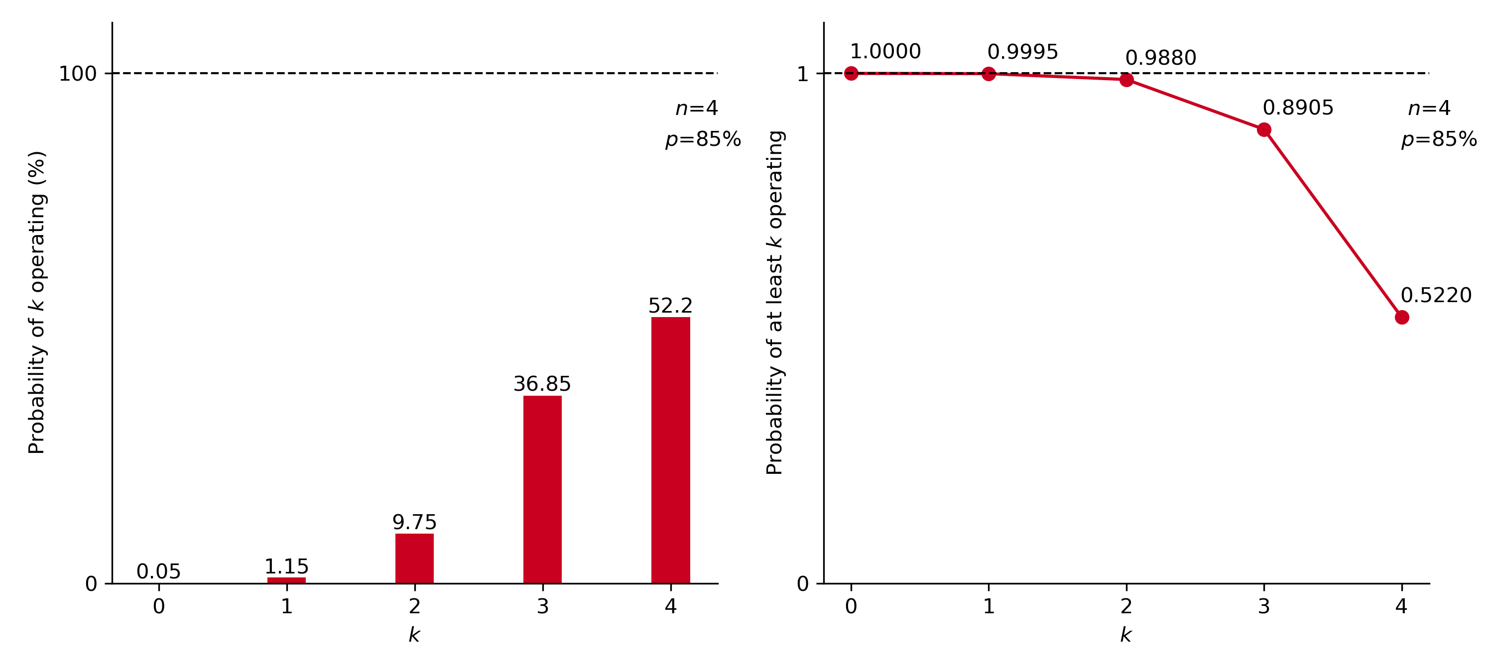
In the example shown in Figure 7, the binomial theorem was applied in a scenario wherein \(n\)=4 shovels were considered, each exhibiting an availability of \(p\)=85%. Both probabilities regarding exactly \(k\) shovels operating, and at least \(k\) shovels operating, at a given time, were calculated. Hence, considering a probability level of 95%, along with the shovels’ availability (85%), a fleet consisting of four shovels would be required to guarantee continuous operation with at least two shovels functioning at all times. This achieves a confidence level of 98.8% (Figure 7), which exceeds the 95% threshold.

Benford’s Law

Benford’s law, also known as the first-digit law, is a categorical variable parametric distribution regarding the probability of a non-zero leading (first) digit in natural numbers spanning many orders of magnitude. In data sets composed of values of four or more digits, the number 1 tends to occur more frequently as the first digit in a sequence of numbers compared to the number 9. The frequency of the first digits, from 1 to 9, closely adheres to a logarithmic relationship (Benford, 1938). The probability (or frequency) of the leading digit can be determined (Benford, 1938):

\[ p(d)=\log _{10}\left(1+\frac{1}{d}\right), \quad d=1, \ldots, 9 \]

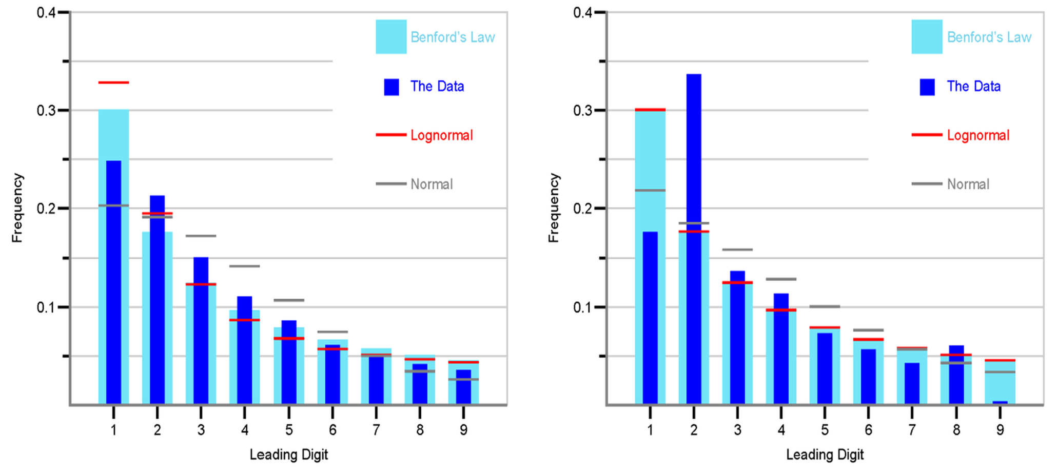
Random numbers uniformly distributed between 0 and 1, as expected, do not conform to Benford’s Law. In Geostatistics, Benford’s law is applied to detect fraud or artifacts in the reported values in the data. A GSLIB-like program (Deutsch, 2016) can be used for assessing the frequency distribution of leading digits and comparing them to Benford’s Law. In addition to examining the distribution of leading digits based on the actual data, both parametric normal and lognormal distributions are established considering the mean and variance of the data values, excluding zeros and missing values, and treating negative values as their absolute counterparts. A random sampling of one million values from each normal and lognormal distribution allows for the evaluation of expected deviations. Benford’s law was applied to some copper and molybdenum data components. The results are shown in Figure 8. Figure 8 exhibits the frequencies represented by bars for both Benford’s Law and the actual data, while the frequencies generated from lognormal and normal distributions are depicted as lines. Some concerns are evident with the molybdenum data, although the lognormal results perfectly match Benford’s law the actual data differs from the expected distribution.

Summary

In Geostatistics, categorical variables are mainly used for the determination of stationary domains for estimation and simulation of continuous variables. Categorical variable modeling serves as a preliminary stage to continuous variable modeling exerting an influence on the accuracy and reliability of resource estimation. The primary objective of this Lesson is to review categorical variables, encompassing their commonly utilized distributions and their behavior when larger scales are considered. This Lesson serves as a preliminary step towards categorical variable modeling, laying the groundwork for the development and application of both object-based and cell-based geostatistical models.

References