Cite this lesson as: Chiquini, A. P., & Deutsch, C. V. (2017). A Simulation Approach to Calibrate Outlier Capping. In J. L. Deutsch (Ed.), Geostatistics Lessons. http://geostatisticslessons.com/lessons/simulationcapping
A Simulation Approach to Calibrate Outlier Capping
Ana Paula Chiquini
University of Alberta
Clayton Deutsch
University of Alberta
February 17, 2017
Learning Objectives
- Appreciate the impact of outlier values on total metal content
- Understand a reliable outlier management method based on simulation
- Increase sensitivity to the importance of outliers
Introduction
Outlier management is important in mineral resources estimation for precious metals and other deposits with highly skewed grade distributions. Assessing the true metal content in such mineral deposits requires special treatment of outliers. Leaving high grades unmanaged in estimation often leads to over estimation of ore tonnage and grade. The high grades may be accurate sample values; however, they may be less spatially continuous than the rest of the grades. A number of geostatistical techniques to deal with outliers in resources estimation of highly skewed distributions variables have been developed.
An approach involving ranking of the outliers has been proposed by Parker (Parker, 1991). The idea is to observe the quantile of the distribution characterized by an abrupt acceleration of the cumulative coefficient of variation and fit a lognormal model to the data above that quantile. Estimation considers a simplified indicator kriging considering that quantile as a threshold and modeling the mean of the distribution tail.
Costa (Costa, 2003) proposed a methodology for treating outliers based on robust kriging that reduces the kriging weights assigned to extreme values by editing these values using the information of the nearby data. This technique uses the kriging variance to determine an acceptable difference between the value to be edited and the weighted median calculated using the local data.
Another alternative is to move the outlier further away to a higher dimension (Deutsch, Boisvert, & Deutsch, 2011). A new dimension is introduced in order to measure and manage the influence of the outlier on the surrounding blocks.
A decomposition of the grade variables has also been proposed (Rivoirard, Demange, Freulon, & Lécureuil, 2013). The idea is to divide the variable into three parts: the truncated grade, a weighted indicator above top-cut grade and a residual. In this approach, the estimation is based on the truncated grade and the indicator cokriging and a separate kriging for residuals. Subdividing the variable improves the structure of the variogram because the indicator and the truncated grades do not keep extreme values.
A common practice is to cut the high grades to a specified maximum value. This cutting level could be determined by experience or reconciliation with production data. An alternative procedure is described here.
Simulation is a robust technique with respect to outlier values; the spatial continuity of the extreme values is not exaggerated by the local weighting of estimation. Kriging is smooth and will likely overstate the grade near outlier values. Nearest neighbour or inverse distance estimation will also give a large weight to nearby outlier values. On the contrary, simulation is designed to compute realizations that reproduce the data, the histogram and the variogram. Although the average of multiple simulated realizations is close to kriging, the average behaviour of multiple realizations may be very different from that of the kriged model, particularly near extreme values.
In this lesson, an outlier management method is proposed that uses simulation to calibrate a cutting level for estimation. Babakhani (Babakhani, 2014) proposed a similar approach where the key idea is to take advantage of the outlier resistance of simulation to determine the cutting level for kriging or any other estimation technique.
Proposed Approach
The steps in the proposed approach are (1) identify the outliers that may be cut; (2) use ordinary kriging or any other estimation technique to identify the volume influenced by these values; (3) use simulation to assess the expected metal content within the volume influenced by the outliers; (4) perform estimation using different cutting levels and choose a cutting level that matches the simulated expected metal content.
The approach proposed here could consider either one outlier at a time or multiple outliers possibly cut to the same value. The simplest alternative is to cut all outliers that belong to the same statistical domain to the same value.
Identifying the Outliers
Prior to managing the outliers, they should be identified. The simplest approach is to choose a maximum value based on experience or past studies. Some other alternatives include:
Probability Plots
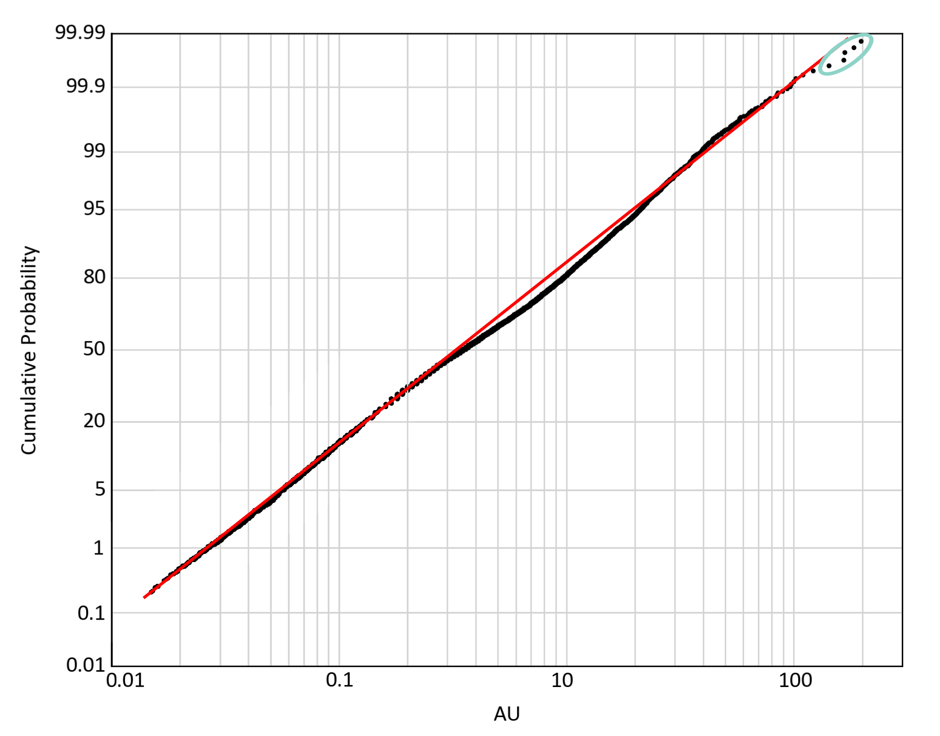
Probability plots are useful tools to identify outliers because each data value is shown individually. The points located at the upper end of the distribution may be considered outliers. A lognormal probability plot is common; the logarithms of the grades are plotted against their cumulative probability on a scaling that would make a lognormal distribution plot as a straight line. An example is shown below. The red line is a possible lognormal distribution. The five values circled in blue are possible outliers, that is, they appear higher than expected relative to the fitted distribution.
Visual Inspection
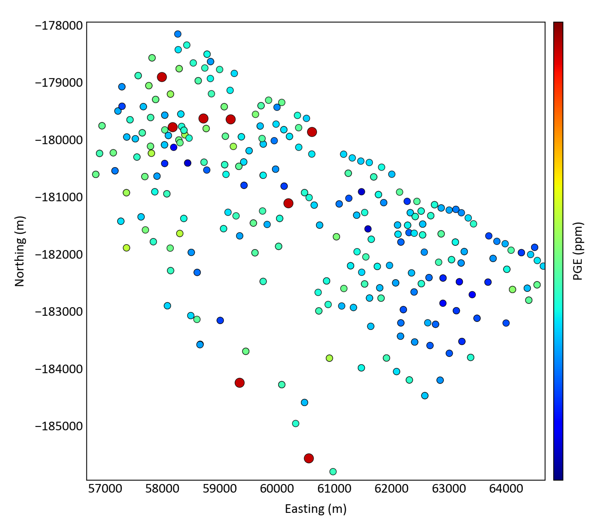
Considering high values in comparison with the entire dataset may not be enough; a comparison with surrounding data should be considered. A high value surrounded by high values may not be an outlier yet a moderately high value surrounded by low values may be considered an outlier. If regions of high values were not considered to be outliers, they would not be cut in subsequent analyses. The figure below shows a plan view of a mineral occurrence with eight outliers identified.
Sensitivity Analysis with Kriging
Performing a sensitivity analysis using ordinary kriging is another way of understanding the outlier distribution and their impact on resources estimation. A number of ordinary kriging runs should be considered with different cutting levels. The objective is to directly observe the influence of the outliers on the estimated metal content. The table below shows an example.
| Top Cut Value (g/t) | Estimation Mean (g/t) | Total Metal Content (Oz) | Metal Content (%) |
|---|---|---|---|
| 27 | 4.11 | 440 | 81 |
| 30 | 4.21 | 450 | 83 |
| 35 | 4.26 | 456 | 84 |
| 45 | 4.36 | 467 | 86 |
| 70 | 4.56 | 488 | 90 |
| no cutting | 5.07 | 543 | 100 |
The experimental variogram may also be sensitive to outliers and robust alternatives may be required. The influence of outliers on other statistics including declustering, the mean, variance and multivariate statistics should also be considered by transformation or sensitivity analysis.
Scale and Compositing
Compositing is a common practice during the resources evaluation workflow. Irregular length assay samples are composited to provide equal-sized data for geostatistical analysis. In general, outliers should be identified on the original assays since some outliers are hidden when composited with other low grade assays. It would be best practice to look for outliers before and after compositing. There is no consensus view, but cutting the original assays seems more common.
Identifying the Volume of Influence
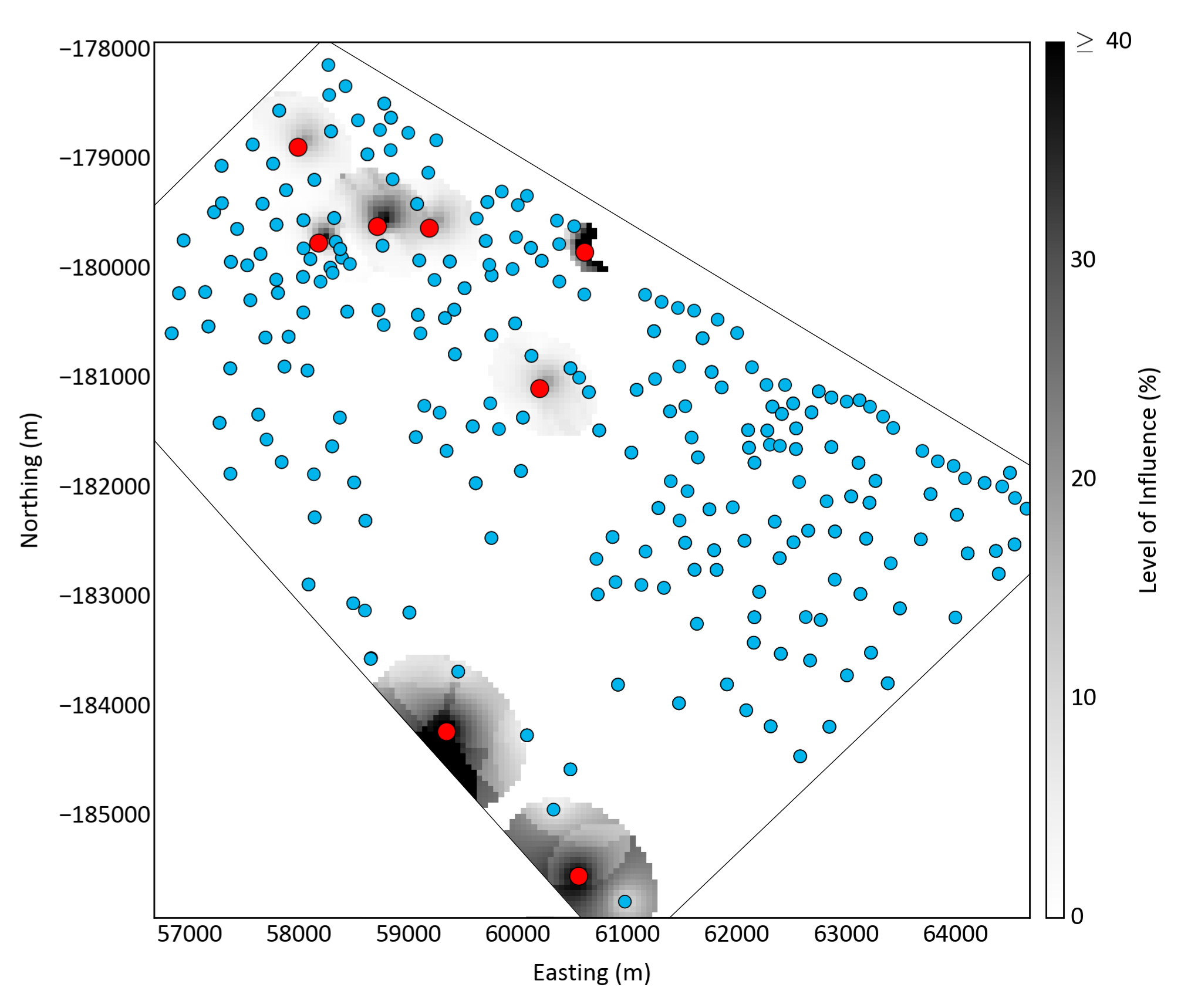
The volume affected by outliers must be identified. One approach is to create an auxiliary data variable that is 100 when an outlier is present and 0 otherwise. This new variable is estimated with the proposed estimation technique and plan. Any volume or block with an estimate different than zero has been influenced by an outlier.
As expected, the volume of influence is strongly dependant on the search radius, number of data used and other details of estimation. The map below illustrates the areas influenced by outliers for a small example; any shading by gray indicates a location influenced by an outlier. The search radius and number of data used are easily seen. Clipping to avoid extrapolation of the volume of influence along the data boundary may be considered.
Simulation
In the proposed approach, simulation is used to determine the uncertainty in the average grade and in the metal content within the volume of influence of outliers. Simulation is a robust technique with respect to outliers; however, outliers can have an impact on the normal score transformation that is required for simulation.
One hundred realizations are simulated to calculate the uncertainty in the metal content inside the volume of influence. The entire volume or the volumes around individual outliers could be considered. The entire volume influenced by outliers is considered here without applying a cutoff grade; this volume is likely all ore. The next step involves estimation considering different cutting levels.
Choosing the Cutting Level
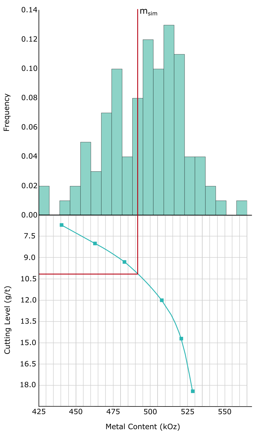
A number of estimates inside the volume of influence are run with different cutting levels. The cutting level is determined so that the estimated metal content matches the mean of the simulated metal content. All data within the domain are used for simulation and estimation; however, the metal content being matched is only calculated in the volume influenced by outliers.
The figure below shows an example. The cutting level chosen in this example is 10.3 g/t, which represents the cutting level that reproduces the mean of the simulated metal content. The distribution of the simulated metal content is well behaved because it represents an average over a large volume.
Final Remarks
The outlier resistance of simulation can be tested by rerunning the simulation with the proposed cutting; the results should not change significantly. This procedure was done for the example above. As shown in the figure below, the uncertainty in the metal content after outlier management (red curve) is very similar to the original results (blue histogram), showing a difference of less than 5% in the total metal content.
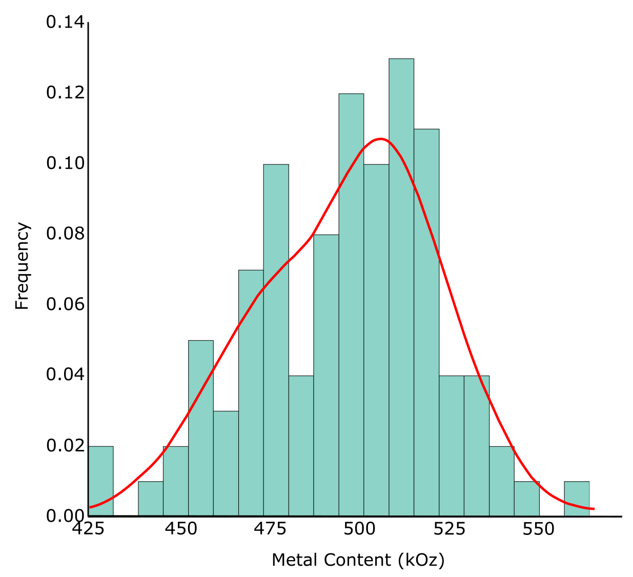
There are many alternative geostatistical techniques to deal with outliers in highly skewed grade distributions variables. Ultimately, reconciliation with production data should be considered to calibrate the outlier management strategy.