Cite this lesson as: Markvoort, H. J. B., & Deutsch, C. V. (2025). Calibrated Multiple Pass Estimation. In J. L. Deutsch (Ed.), Geostatistics Lessons. Retrieved from http://www.geostatisticslessons.com/lessons
Calibrated Multiple Pass Estimation
Hunter John Brine Markvoort
University of Alberta
Clayton V. Deutsch
University of Alberta
December 11, 2025
Learning Objectives
- Recall how change of support predicts block variance
- Learn how to calibrate Multiple Pass Estimation (MPE) to reproduce the correct block variance
- Apply a structured workflow to achieve correct smoothing with variable data density
Introduction
High-resolution simulation is regarded as the most accurate and precise modern approach for resource estimation. Simulation captures geological uncertainty and provides a realistic representation of grade variability. However, software limitations, specialized training requirements, and time constraints continue to restrict its use in routine modelling. As a result, kriging remains the most commonly applied estimation technique in the mining industry (Rossi & Deutsch, 2013). Within kriging-based workflows, Multiple Pass Estimation (MPE) is the standard approach used in feasibility and pre-feasibility studies. A review of more than 200 recent NI 43-101 reports (SEDAR) shows that MPE is applied in over 25% of mining projects (Xia & Deutsch, 2022). Despite its widespread use, there are no guidelines for defining or tuning search parameters within the MPE framework. In practice, parameter selection depends on the practitioner’s experience, leading to inconsistent results between models.
Ordinary Kriging (OK) dominates resource estimation. Search parameters should be adjusted to ensure the model is fit for purpose. A short-term final model considers all nearby relevant data (twenty or more data) for the best possible conditionally unbiased model. A long-term resource model, constructed without the benefit of the final data, must be calibrated to generate the correct resource estimate. The calibration depends on the data spacing where less data are used when kriging in areas of wide data spacing. Multiple search passes or multiple pass estimation (MPE) are considered to partition each domain into regions of different data spacing.
This lesson presents a structured framework for calibrating MPE based on change-of-support theory. The approach links each pass to a variance reduction factor \(f\) derived from the variogram and block geometry. By calibrating each pass to reproduce the expected variance at the SMU scale, MPE becomes a reproducible and practical estimation method that improves the reliability and consistency of long-term resource models.
The calibration framework presented here is most applicable for large open-pit operations where SMU-scale smoothing strongly influences tonnage and grade forecasts. The framework is less applicable in highly selective underground settings. In such environments, minimizing conditional bias often takes precedence over matching the exact change-of-support target, and practitioners typically balance these considerations based on expected mining selectivity and future data availability.
Change of Support
Samples used for mineral resource estimation represent very small volumes relative to the Selective Mining Unit (SMU). As grades are averaged over larger volumes, high and low values combine, reducing variability; block-scale distributions are therefore less variable and more symmetric than sample-scale distributions (Parker, 1980). This relationship between data support and block support is known as change of support. Modelling change of support is essential for estimating recoverable resources. It predicts how grade distributions evolve with increasing volume using only composite-scale data. A comprehensive description of change-of-support models is provided in Harding & Deutsch (2019).
Selecting The SMU Size
The Selective Mining Unit (SMU) is a block size that represents the selectivity and recoverable reserves that will be obtained at the time of future mining. The SMU block size considers mining equipment, bench height, available data at the time of grade control, operational conditions such as blast movement, and geological conditions such as visual control and spotting in the pit. SMU blocks are not actually mined; high resolution dig limits will be mined with the greatest precision possible. Yet, the SMU block size is intended to provide a resource model with the correct smoothing, that is, a model that will reconcile well to future mining.
Reconciliation to actual production is perhaps the best way to select the SMU size. Although accurate, this method is not always possible. Professional judgement and experience could be used, but this is quite subjective. A widely applied alternative is the comparative approach of Leuangthong, Neufeld, & Deutsch (2003), which selects the SMU by matching aggregated tonnes, grade, and metal to a reference simulated grade-control model. The detailed procedure is beyond the scope of this lesson; interested readers are referred to the original paper.
Variance Correction Factor
The variance correction factor (VCF), denoted as \(f\), quantifies the reduction in variance when moving from point support to block support. It is the ratio of the SMU block variance to original data variance (Parker, 1980). The VCF is derived from the variogram by averaging semivariance values over the SMU volume. This calculation is expressed as:
\[ f = \frac{\sigma^2 - \overline{\gamma}(V, V)}{\sigma^2}, \]
where \(\sigma^2\) is the data variance and \(\overline{\gamma}(V, V)\) is the average variogram value over the SMU support volume \(V\) (Harding & Deutsch, 2019). There are many software tools to compute \(f\) for a given variogram model, block geometry, and discretization. The value of \(f\) provides a direct measure of how much variance is retained at block scale. High \(f\) values (e.g., 0.8–0.9) indicate that SMU blocks retain most of the sample-scale variability. This occurs when blocks are small or the spatial continuity is strong relative to block size. Low \(f\) values (e.g., 0.3–0.5) imply that block-scale variance is much lower than point-scale variance. This corresponds to large SMUs or short variogram ranges where substantial smoothing occurs.
Variance of Estimate
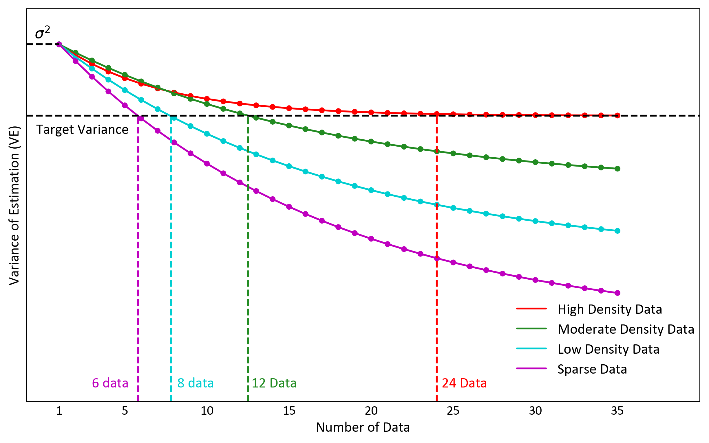
In geostatistics, the minimized estimation variance is known as the kriging variance. This variance measures the expected squared difference between the true and estimated values. The variance of the estimate (VE) is a distinct concept. It is the variance of the kriged block values. VE is controlled by the search configuration and data density. Searches with more data produce smoother results and lower VE, while searches with fewer data produce more variable results and higher VE. Figure 1 shows that VE also depends on data density: as data becomes sparse, fewer samples are required to attain the same VE(Markvoort & Deutsch, 2025a). This relationship is important for calibrating kriging passes.
Calibrated Multiple Pass Estimation
A single-pass estimation strategy applies the same search parameters everywhere, regardless of data density. This often causes under-smoothing in dense zones and over-smoothing in sparse zones, leading to inconsistent tonnes, grades, and metal outcomes. Figure 2 shows a simplified scenario with four zones of increasing drill spacing. Each zone represents different data density requiring distinct search parameters to achieve the correct smoothing. A single-pass estimation cannot account for this variation, while multiple pass estimation adapts to each zone.
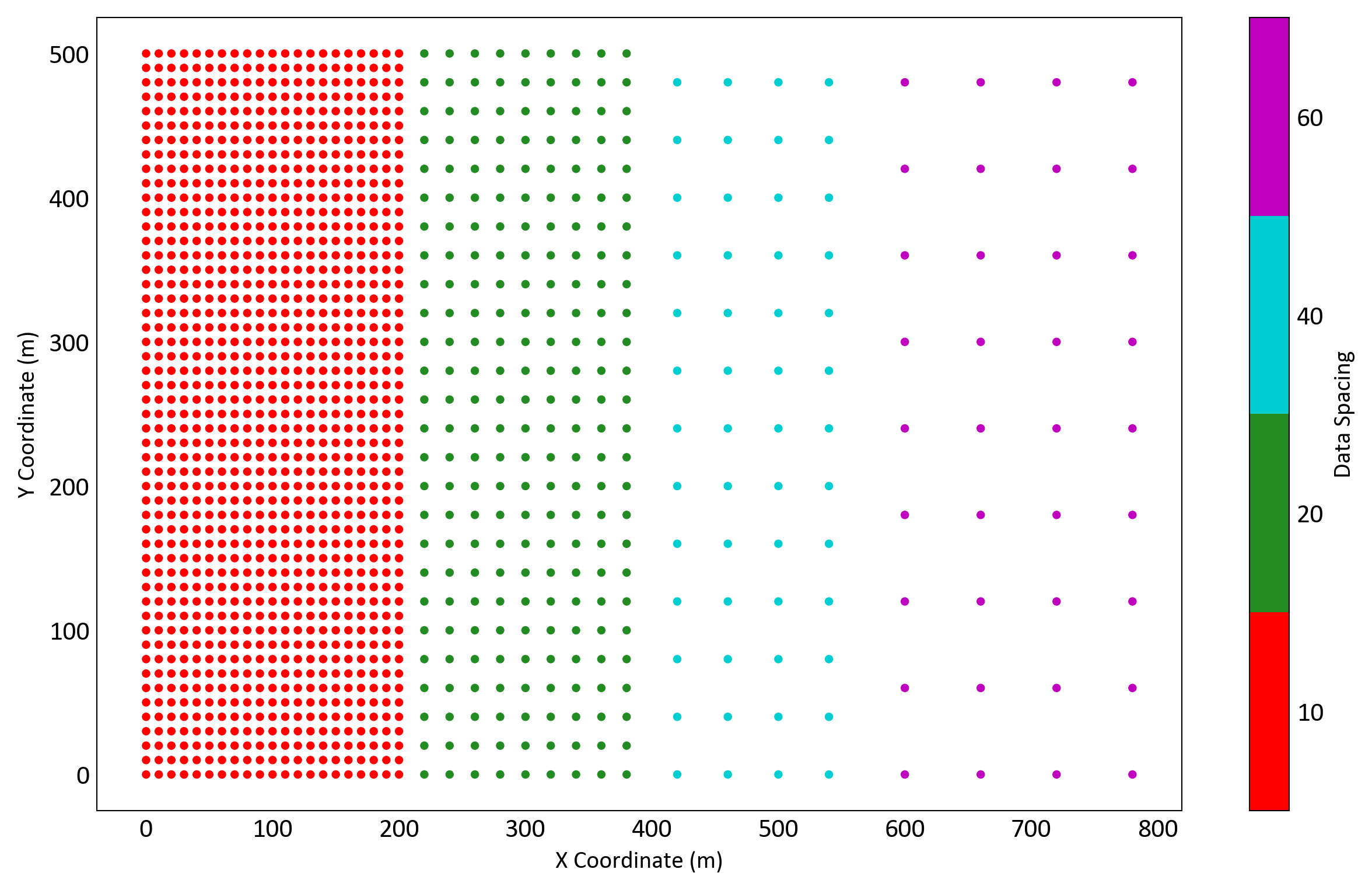
These four zones are colour-coded to match those shown in Figure 1, which illustrates how the variance of estimation (VE) behaves as a function of both data spacing and number of samples used. In dense areas (red), many samples are required to reach the target variance, while in sparse areas (purple), only a few are needed. The combination of these two figures helps visualize why a single global search cannot achieve target smoothing across variable data density.
Limits of Smoothing Behaviour
Two end-member cases demonstrate the effect of incorrect smoothing. A single-pass large-search (SPLS) approach over-smooths: variability is suppressed, and results tend toward the mean. When the cutoff lies below the mean, smoothing inflates ore tonnes but reduces grade; when above the mean, it reduces tonnes. At the other extreme, nearest-neighbour (NN) estimation applies no smoothing, reproduces data-scale variance and consistently reports fewer ore tonnes and higher grades than expected at the block scale. These examples show the consequences of using uncalibrated search parameters. The calibrated Multiple Pass Estimation (MPE) framework overcomes this by tuning each pass to reproduce the correct variance at SMU support.
Calibrated MPE Concept
The calibrated MPE framework addresses the challenge of variable data density by applying successive searches with tailored parameters. Calibration of passes follows change-of-support principles. The variance correction factor (\(f\)), defined earlier, represents the ratio of block variance to point variance. The VE of the NN estimates serves as a proxy for point-support variance. NN applies no smoothing and assigns one sample value to each block, reducing the influence of clustered drilling and providing a practical point-support reference for MPE calibration. For each pass, the VE of the kriged estimates is compared to the NN VE for the same blocks. The ratio of these two variances is then compared to \(f\), with the goal of achieving agreement within 5–10%. Each pass is tuned through adjustments to the number of samples, search radius, and per-drillhole limits(Markvoort & Deutsch, 2025a). After each pass estimates are assigned to blocks and excluded from subsequent searches. Later passes only fill areas left un-estimated. This stepwise strategy adapts to changing data spacing; dense zones use more samples to preserve variability, while sparse zones use fewer samples to avoid excessive smoothing. The procedure balances selectivity and stability across the deposit, creating estimates that are consistent with change-of-support theory (E. Isaaks, 2004). The following procedure formalizes the calibration workflow step by step.
Calibrated MPE Workflow
Define the number of passes Identify distinct zones of data spacing within each domain. The number of passes corresponds to the number of distinct spacings. There are normally 2 to 5 passes.
Note the expected block proportions per pass Identify the approximate fraction of blocks expected to fall within each spacing zone. These proportions serve as a reference during calibration: if a pass estimates far more or far fewer blocks than expected, the search radius or minimum number of samples are adjusted.
Perform nearest neighbour (NN) estimate Generate NN estimates for each domain. These allow the representative point support variance to be calculated for each pass in subsequent calculations.
Compute the \(f\) coefficient Calculate the variance correction factor \(f\) for each domain. The \(f\) coefficient depends on the variogram, SMU size, and discretization geometry, and is therefore constant for a given domain.
Perform the first pass Begin with the highest density zone. Use the search radius to constrain the percentage of blocks estimated and minimum/maximum samples to tune the VE.
- A general rule is to set the minimum number of samples at approximately 75% of the maximum (E. H. Isaaks & Srivastava, 1989). This keeps the min–max ranges narrow to isolate specific data spacings rather than blending across zones. The minimum number of samples could be set equal to the maximum, but some tolerance seems to work better.
- Limit the number of samples per drillhole to 2 or 3 to reduce artifacts due to the string effect
- Limit the number of samples by octant to avoid unnecessary artifacts.
Calibrate each pass by checking the variance ratio The calibration target is:
\[ \frac{\mathrm{Var}(Z^*)}{\mathrm{Var}(Z_{\text{NN}})} \approx f_{\text{COS}} \]
where \(\mathrm{Var}(Z^*)\) is the VE of kriged SMU estimates and \(\mathrm{Var}(Z_{\text{NN}})\) is the VE of NN estimates for the same blocks.
Adjust the number of samples:
- Reduce the number of samples used if the ratio is too low (increase VE).
- Increase the number of samples used if the ratio is too high (decrease VE).
- Adjust the search radius to increase or decrease the proportion of blocks estimated so that it matches the expected block percentage for that pass.
- Continue iterating until both the variance ratio and the target percentage of blocks estimated are satisfied.
Repeat for subsequent passes and domains Hard-code estimates from previous passes and continue calibration for remaining blocks, targeting progressively lower data densities. Maintain the ratio within 5–10% of \(f\) for each pass. Use larger search radii in later passes if necessary to ensure full coverage. Repeat the procedure for each domain independently, as the variogram, data distribution, and \(f\) coefficient are domain-specific.
Estimate using the calibrated MPE Apply the calibrated search parameters across all passes and domains to complete the Calibrated MPE workflow. The final model reproduces the expected variance at the SMU scale and maintains consistency across zones of varying data density.
The calibrated multi-pass framework provides a systematic approach to control smoothing across zones of variable data density. Note that drill holes are often clustered in high grade areas and those areas are more variable than low grade areas. This is why the variance reduction is considered relative to the variance of the NN estimates. By aligning the variance of kriged estimates with the change-of-support target, the procedure avoids the biases of oversmoothing and undersmoothing. The following case study demonstrate how the calibrated MPE compares with a single pass large search and NN estimates in practice.
Case Study: Misima Dataset
Reference Blast-Hole Model
A reference blast-hole model is constructed from Misima blast-hole data (Vasylchuk & Deutsch, 2017). A 5 m block grid is upscaled to a 10 × 10 × 10 m Selective Mining Unit (SMU) and aggregated into monthly production volumes of approximately 500,000 t. Ore tonnes are calculated using a fixed dry bulk density of 2.25 t/m³ and a cutoff grade of 0.30 g/t Au. The blast-hole model reports 411.8 Mt of ore at an average grade of 0.76 g/t Au, containing 10.1 Moz Au, distributed across 856 production volumes.
The blast hole model serves as a final estimate, with no further information expected. It classifies material as ore or waste with direct economic consequences; the emphasis is on minimizing conditional bias, mean squared error, and misclassification of ore and waste. Best practice is to apply Ordinary Kriging with a large search to reduce estimation error and conditional bias, ensuring that all available data contribute to the estimate (Deutsch & Deutsch, 2015).
Exploration Dataset
The exploration dataset is sampled directly from the blast-hole data. A spatial zoning step classifies a regular grid by mean grade and applies a majority filter to form coherent Measured, Indicated, and Inferred zones. Zone-based thinning then enforces realistic spacings (approximately 30 m, 60 m, and 120 m) while retaining full vertical profiles for selected drillholes. The resulting dataset reproduces large-scale grade trends while reflecting the drillhole density expected in exploration programs. Detailed procedures for estimating the blast hole model and creation of the exploration dataset can be found in Markvoort & Deutsch (2025b).
The blast-hole model provides the production reference, while the exploration dataset supplies the input data for the interim estimation models. Consistent cutoff, density assumptions, and variography are applied to both datasets to isolate the effect of the estimation method rather than differences in variogram modeling or data configuration. Results are reported by domain at a cutoff grade of 0.3 g/t Au. The analysis highlights how oversmoothing and undersmoothing create systematic biases, and how calibration in the MPE framework provides balanced outcomes consistent with change-of-support theory.
Calibrated Multiple Pass Estimation
The calibrated multipass approach is applied to the Misima dataset. Each domain is analyzed separately, with passes defined according to drillhole spacing. NN estimates provide the point-support variance reference, while the variance correction factor (\(f\)) sets the calibration target.
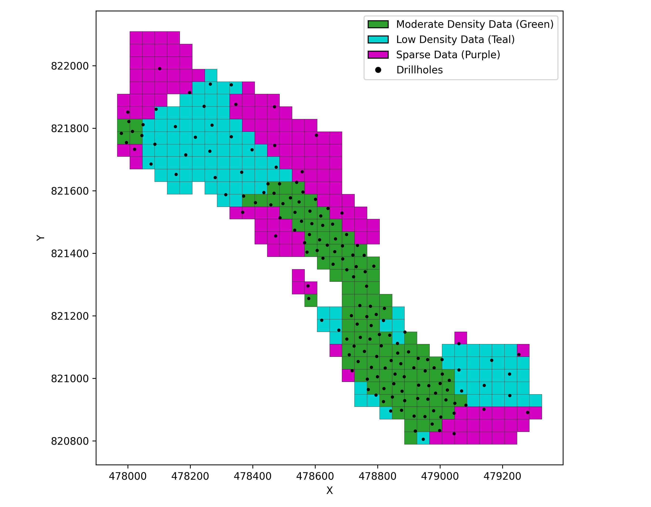
Step 1: Define the number of passes Identify distinct zones of drillhole spacing within each domain. The number of passes corresponds to the number of distinct spacings. In this study, three passes are defined to represent 30 m, 60 m, and 120 m spacing (Markvoort & Deutsch, 2025b). Figure 3 visualizes the three spacing zones that define the MPE passes and the retained drillholes used for calibration in domain 1. In practice, the number of passes depends on the dataset and is determined by examining spatial distributions within each domain.
Step 2: Note the expected block proportions per pass Block proportions are determined by counting the number of SMUs in each domain and applying the percentage assigned to each pass. Table 1 summarizes the distribution for the Misima grid, which contains 273,581 SMUs in total. These targets set the expected number of blocks per pass and serve as the benchmark for calibrating search parameters in each domain.
| Domain | Total SMUs | Pass 1 (30%) | Pass 2 (40%) | Pass 3 (30%) |
|---|---|---|---|---|
| 1 | 146,725 | 44,018 | 58,690 | 44,018 |
| 2 | 78,086 | 23,426 | 31,234 | 23,426 |
| 3 | 24,067 | 7,220 | 9,627 | 7,220 |
| 4 | 13,280 | 3,984 | 5,312 | 3,984 |
| Total | 262,158 | 78,648 | 104,863 | 78,648 |
Step 3: Perform NN estimation Generate an NN model for each domain to provide the point-support variance reference. The search ellipsoid is defined from the variogram anisotropy (E. H. Isaaks & Srivastava, 1989).
Step 4: Compute the \(f\) coefficient For each domain, calculate the variance correction factor (\(f\)) for each domain. Table 2 summarizes the results for the domain 1, showing both the pass targets and the \(f\) coefficient window used in calibration.
| Domain | \(f_{target}\) | \(f_{low}\) | \(f_{high}\) |
|---|---|---|---|
| 1 | 0.299 | 0.269 | 0.329 |
| 2 | 0.262 | 0.236 | 0.288 |
| 3 | 0.255 | 0.230 | 0.281 |
| 4 | 0.430 | 0.387 | 0.473 |
Step 5: Estimate a pass and compute the variance ratio Run the pass with initial search parameters and calculate the variance ratio, \(\mathrm{Var}(Z^*)/\mathrm{Var}(Z_{\text{NN}})\). Compare the result to the target \(f\) coefficient (Table 2).
Step 6: Calibrate each pass Iteratively adjust the search parameters until both the variance ratio and block count fall within their targets. Three parameters are adjusted during calibration: search radius, minimum number of data, and maximum number of data. Together they influence two key outcomes:
The number of blocks estimated (block coverage)
The degree of smoothing, expressed as the variance of the estimates (VE).
Block coverage is controlled by the search radius and the minimum number of data. The variance is influenced by both the minimum and maximum number of data. The maximum number of data affects only the variance, whereas the minimum number of data influences both variance and block coverage. The search radius mainly controls block coverage but can also slightly affect variance depending on data spacing and variability. Recognizing these relationships allows the modeler to adjust parameters deliberately, using the minimum and search radius to reach the desired block coverage, and the maximum to refine the variance toward the target f coefficient:
- If the ratio is below the lower bound of the \(f\) window (too much smoothing), increase VE by reducing the number of samples (lower the minimum and maximum).
- If the ratio is above the upper bound (too little smoothing), decrease VE by requiring more samples (raise the minimum and maximum).
- Adjust the search radius to estimate the target number of blocks. Note that the block coverage and smoothing are linked.
- Re-evaluate and repeat, making small adjustments, until both the variance ratio and block count fall within tolerance.
| Iter | \(n\) blocks | Min–Max | Buffer | Ratio | Notes |
|---|---|---|---|---|---|
| A | 90,349 | 8–10 | 2.50 | 0.279 | Within \(f\) window, but too many blocks. - Tighten search. |
| B | 44,477 | 10–12 | 1.85 | 0.247 | Correct block count, but ratio too
low. - Use fewer samples. |
| C | 44,182 | 8–10 | 1.70 | 0.274 | Within \(f\) window, correct block count. - Accept Pass 1. |
Step 7: Repeat for subsequent passes and domains Once a pass is calibrated, the estimates are locked in and the next pass is considered. Each pass aims to satisfy both the variance ratio and block coverage criteria. Later passes require larger search radii. The procedure is repeated for each domain. The calibrated results are summarized in Table 4, and a spatial verification is shown in Figure 4.
In most cases, the variance ratio falls within the \(f\) coefficient tolerance window. Small domains with few data (e.g.,domain 4) are more difficult to calibrate. In this case, only two passes are applied, with the second pass unable to be tuned into the \(f\) window. Parameters are therefore chosen to balance coverage and stability, representing the best achievable calibration under the data constraints.
| Domain | \(f_{\text{target}}\) | \(f_{\text{low}}\) | \(f_{\text{high}}\) | Pass | \(n_{\text{target}}\) | \(n\) | Ratio | Min | Max | Max DH | Buffer |
|---|---|---|---|---|---|---|---|---|---|---|---|
| 1 | 0.299 | 0.269 | 0.329 | 1 | 44,018 | 44,182 | 0.274 | 8 | 10 | 3 | 1.70 |
| 2 | 58,690 | 59,004 | 0.310 | 7 | 7 | 3 | 2.70 | ||||
| 3 | 44,017 | 43,539 | 0.301 | 6 | 6 | 2 | 20.0 | ||||
| 2 | 0.262 | 0.235 | 0.288 | 1 | 23,426 | 22,592 | 0.231 | 8 | 9 | 3 | 2.5 |
| 2 | 31,234 | 33,508 | 0.268 | 6 | 7 | 3 | 4.0 | ||||
| 3 | 23,426 | 21,986 | 0.261 | 5 | 6 | 2 | 20.0 | ||||
| 3 | 0.255 | 0.230 | 0.281 | 1 | 7,220 | 7,298 | 0.236 | 8 | 8 | 3 | 3.5 |
| 2 | 9,627 | 9,450 | 0.286 | 7 | 8 | 3 | 5.5 | ||||
| 3 | 7,220 | 7,319 | 0.475 | 3 | 4 | 3 | 12.0 | ||||
| 4 | 0.430 | 0.387 | 0.473 | 1 | 3,984 | 8,867 | 0.394 | 3 | 3 | 2 | 2.5 |
| 2 | 5,312 | 4,413 | 0.325 | 3 | 3 | 3 | 12.0 |
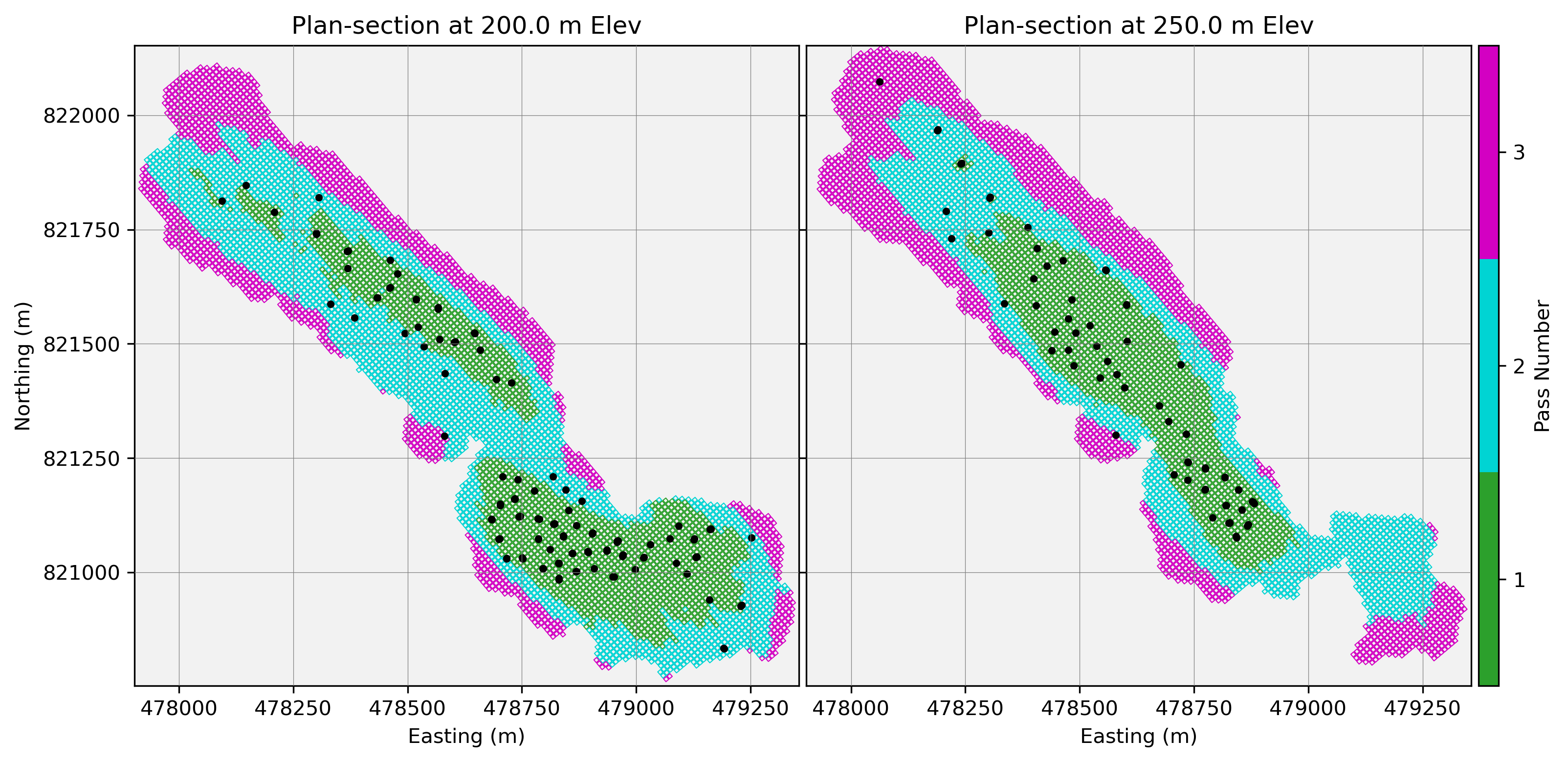
As a final verification step, the calibrated MPE passes are visualized to confirm that block assignment by pass aligns with expectations. Figure 4 shows a set of plan sections through domain 1, where Pass 1 (green) occupies the highest density zones, Pass 2 (teal) extends to intermediate spacing, and Pass 3 (purple) covers the sparsest areas. This check ensures the calibration results are spatially coherent. In practice, such plots are also valuable during calibration, providing visual feedback on how adjustments to search radius and sample limits affect block assignment.
Step 8: Estimate using the calibrated MPE Apply the calibrated search parameters in the MPE framework. Each pass runs sequentially, with estimates from earlier passes hard-coded before later passes are applied. The final calibrated MPE model reproduces variance consistent with the \(f\) coefficient target at the SMU scale and provides a reliable foundation for reconciliation.
Results
The three estimators show distinct smoothing behaviours when compared with the blast-hole model. The grade–tonnage curve (Figure 5) illustrates these differences clearly. SPLS over-smooths and shifts estimates toward the mean, which increases ore tonnes and lowers ore grades across a range of cutoffs. NNM preserves point-scale variability, produces more extreme values, and yields higher grades but fewer tonnes. The calibrated MPE sits between these extremes and tracks the BHM curve closely, indicating appropriate selectivity at the SMU scale.
These behaviours appear directly in the pass-by-pass histograms (Figure 6). SPLS compresses the grade distribution and suppresses high-grade tails. NNM exaggerates variability, preserves extreme values, and shifts material above the cutoff. MPE reproduces the BHM distribution more faithfully in each pass, maintaining both the central tendency and the upper tail. The histograms demonstrate how smoothing differences at each pass accumulate into the global patterns shown by the GT curve.

These visual patterns align with the numerical results. Considering the cutoff grade, SPLS inflates raw grades by 5–24% across domains, raising the total mean grade by 17%. NNM reduces raw grades by 5–12%, reflecting its greater local variability. MPE remains closest to the reference, with raw grades within ±9% in the larger domains and a total deviation of only +2%. After applying the 0.30 g/t cutoff, the contrasts become more pronounced. SPLS understates ore grades by 5% in total, while NNM overstates grades by 36%. MPE again stays closest to the BHM, reproducing the total ore grade within −1%.
The same pattern appears in ore tonnes. Considering the cutoff grade, SPLS inflates tonnes by 30–110% across domains (a total increase of 36%). NNM understates tonnes by 28–37% (a total reduction of 32%). MPE estimates total ore tonnes within +7% of the reference. Contained metal reflects the combined effect of grade and tonnage. SPLS overstates metal by 15–32% per domain (a total increase of 28%). NNM understates metal by 12–18% (a total decrease of 8%). MPE remains closest to the BHM, reproducing total contained metal within +5%.
Taken together, these results show a consistent and expected pattern. SPLS over-smooths and draws material across the cutoff, producing higher tonnes and lower grades. NNM under-smooths and exaggerates local variability, producing higher grades but fewer tonnes. The calibrated MPE achieves the intended level of smoothing and reproduces BHM behaviour most faithfully across all metrics.
Discussion
This lesson demonstrates how calibration reduces the subjectivity in Ordinary Kriging. By targeting the change-of-support variance, the calibrated multiple-pass estimation approach ensures that each pass produces the correct level of smoothing for the data spacing present. Calibration reduces subjective choices about search radii and data limits. The workflow ties each search configuration to a measurable variance target. This produces estimates that are defensible, repeatable, and theoretically grounded, improving consistency between practitioners and confidence in model-based decisions. The logical next step extends these principles from domain-level calibration to block-level calibration. Local Search Optimization applies the same variance-targeting approach at each block, adjusting the search configuration locally so that the variance of estimate matches the expected support (Silva & Deutsch, 2025). This progression, from global calibration to local calibration, moves Ordinary Kriging toward a fully automated and theoretically consistent estimation method.