Learning Objectives

• Understand the importance of discretization in geostatistical modeling of blocks
• Highlight factors that influence the recommended discretization level
• Demonstrate sensitivity to the number of discretization points

Introduction

Spatially correlated random variables are assigned to grid blocks to assess resources, reserves, and for engineering design. Grid blocks are discretized to account for the small scale of data relative to the block size. Block discretization is practically important in geostatistical workflows. In the mining and petroleum industries, kriging and simulation techniques are used to estimate and simulate random variables that represent grid blocks. In block kriging, the data-to-block average covariances are calculated by discretizing the block with a set of locations. Similarly, in geostatistical simulation, the blocks are represented by a set of simulated points. Geostatistical simulation takes place at the scale of the data; however, it is not practical to exhaustively simulate at the scale of the data, as this would require an unreasonable computational cost and is not required in any case. A reasonable number of discretization points will suffice.

This lesson demonstrates some factors that influence the choice of the discretization level to reasonably estimate effective block properties.

Discretization

Discretization is the process to subdivide space into a series of points or the method used for transforming a coarse grid (structured or unstructured) into a set of conforming fine grids (Manchuk, 2010). Each discretization point or node represents a volume that is an integral part of the grid block under consideration. In geostatistical simulation, the act of grid refinement and point modeling is fundamental to capture the variations of rock properties within the target grid. The discretization of blocks is similar to concepts in other numerical methods including computational fluid dynamics.

For illustration, consider a 2-D block of dimension \(l\), discretized by \(n\) by \(n\) points, where \(z_{ij}\) is the block property value at each discretization point, \(i,j=1,\ldots,n\), representing the position in the block. Note that the discretization points are evenly distributed in the 1, 2 or 3-D volume or regular grid (Deutsch & Journel, 1997).

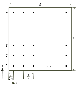
The average block property is the upscaled average property of the block given as:

\[\overline{z}(n)\ = \frac{1}{n^{2}}\sum_{i=1}^{n}\sum_{j=1}^{n}z_{i,j}\]

The number of discretization points required to reasonably calculate block properties must be specified. This depends on several factors including: (1) the block dimension, that is, 1, 2 or 3-D, (2) the spatial correlation, that is, the variogram, and (3) the nature of upscaling, for example, linear averaging or flow based upscaling. Geological properties describe the nature and predict the performance of a geological site, for example, a reservoir. Properties including mineral grade, thickness, porosity and fluid saturations are scalar (static) properties, while permeability is a vector/tensor (dynamic) property.

In what follows, both numerical and analytical methods are applied to discretize a grid block and upscale the property of interest. The discretization error is assessed and used as a basis for recommending a reasonable discretization level for effective block property estimation.

Discretization Error

To numerically assess discretization error, consider a 2-D block of dimension \(100\)x\(100\)x\(1\). An unconditional standard Gaussian simulation is performed. The block is discretized with \(20\) different levels of discretization: \(n=1,\ldots,20\). An \(n\) by \(n\) discretization contains \(n^2\) points in the block. Since scalar properties average linearly, grid point values are scaled up arithmetically to obtain the block property \(\overline{z}(n)\). The discretization error relative to the reference grid block, \(e(n)\), is calculated for each discretization:

\[e(n)=z(n) - z_{ref}, \;\; n=1,\ldots,20\]

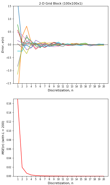
Plots of the error for ten realizations are shown in the figure below. To summarize the error in estimating the block property, multiple (\(L=200\)) realizations of the model are generated and the mean squared error (\(MSE\)) is calculated:

\[MSE(n) =\frac{1}{L}\sum_{l=1}^{L}e_{l}(n)^2,n=1,\ldots,20\]

As expected, the estimation error decreases with an increasing number of discretization points.

An analytical approach could be used to assess the discretization error. The mean squared error \(MSE\) is:

\[ \begin{aligned} MSE(n) &=E\left \{[\overline{z}(n) - \overline{z}(\infty)]^{2} \right \} \\ &=E\left \{ \overline{z}^{2}(n) \right \} - 2E\left \{ \overline{z}(n) \cdot \overline{z}(\infty) \right \} + E\left \{ \overline{z}^{2}(\infty) \right \} \end{aligned} \]

Where \(\overline{z}(\infty)\) is the reference block average with an infinite or very large discretization. Assuming the mean is zero, \(E\left\{\overline{z}^2(n)\right\}\) is the variance of the block property, calculated as:

\[ E\left\{\overline{z}^2(n)\right\}=\frac{1}{n^{4}}\sum_{i=1}^{n}\sum_{j=1}^{n}\sum_{k=1}^{n}\sum_{m=1}^{n}E\left \{ z_{i,j} \cdot z_{k,m} \right \} \]

Where \(i,k=1,\ldots,n\) are \(X\) position indices and \(j,m=1,\ldots,n\) are \(Y\) position indices. The expected product of property values are covariances:

\[ E\left \{ z_{i,j} \cdot z_{k,m}\right \}=Cov\left\{z_{i,j} \cdot z_{k,m}\right\} \]

The error from the analytical approach is the same as the numerical simulation. The analytical approach is applicable to variables that average linearly.

Block Dimension

The error is now assessed for a scalar property of 1-D and 3-D grid blocks. Plots of the discretization error for the 1, 2 and 3-D cases are shown below. The result shows that a high dimensional model yields less error for the same discretization level \(n\). This is expected since for the same \(n\), a 3-D block requires \(n^3\) points to model the block property, while a 1-D block only requires \(n\) points; more discretization points implies high resolution and reduced error. Note that the error does not depend simply on \(n\) or the total number of points.

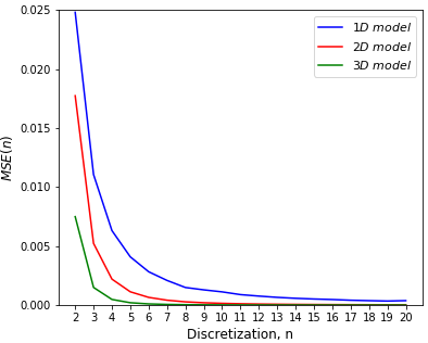
These results show that a reasonable discretization level would be \(8\) in 1-D, \(5\) by \(5\) in 2-D, and \(4\) by \(4\) by \(4\) in 3-D. These values are chosen by the low absolute error and the low relative improvement for higher levels of discretization.

Spatial Correlation

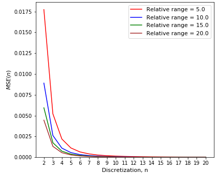
The importance of the variogram as a factor in choosing the required discretization level is studied by modeling the values in the 2-D block model with varying variogram range \(a\_h_d\) from 5.0 to 20.0 times the block size of the model. The result below shows that the \(MSE\) decreases with an increasing variogram range. The suggested \(5\)x\(5\) appears reasonable for all variogram range values.

Zonal Anisotropy

Most geological formations show different spatial continuity in different directions. In geometric anisotropy, the variograms in the directions of maximum and minimum continuity have similar shape and sill but different ranges of correlation. Zonal anisotropy is a special case of geometric anisotropy where the range of correlation in one or two directions exceeds the domain size, which leads to a directional variogram that appears not to reach the sill or variance (Pyrcz & Deutsch, 2014). Sensitivity analysis with variograms showing zonal anisotropy confirm the results shown above - the error is less for a longer range and the discretization levels of \(5\) by \(5\) in 2-D and a \(4\) by \(4\) by \(4\) in 3-D remain reasonable.

Average Variogram Calculation

A drill hole or point scale data distribution of a property of interest has a larger variance than the block distribution of the same property. A global block or selective mining unit (\(SMU\)) distribution can be inferred from a representative distribution of point scale data (Rossi & Deutsch, 2014). The reduction in variance at a block of size \(V\) is quantified by the average variogram \(\overline{\gamma}(V,V)\). The block is discretized into \(n\) points and the variogram \(\gamma(h_{i,j})\), \(i,j=1,\ldots,n\) values are averaged. A rule of thumb is that a \(5\) by \(5\) by \(5\) discretization within a 3-D \(SMU\) is sufficient to obtain a robust estimate of \(D^2(v,V)\) (Rossi & Deutsch, 2014). The results of this study are consistent with this and show that \(5\) by \(5\) in 2-D and \(4\) by \(4\) by \(4\) in 3-D are reasonable discretization levels to use.

Composite Size

Drill hole samples are often averaged into regular length composites. The chosen composite length often depends on the anticipated selective mining unit \(SMU\). In open pits mining, the selectivity in the vertical dimension is generally fixed at the bench height, while in the case of underground mines, selectivity is a function of the mining method (Rossi & Deutsch, 2014). The discretization level chosen to estimate the property of interest in the \(SMU\) will depend on the composite length, among other factors. For example, consider a \(20\)x\(20\)x\(20\)m \(SMU\) with \(10\)m vertical drill hole composites. The discretization \(n\) in the vertical dimension is the ratio of the block vertical dimension to the composite length, that is, \(n=2\). Hence, a \(4\) by \(4\) by \(2\) discretization level would be reasonable for the \(SMU\).

Nature of Upscaling

Geostatistical methods generate reservoir descriptions at a high resolution. Upscaling is applied to compute effective properties at a larger scale that capture the influence of the smaller scales. The accuracy of such effective properties, as applied to flow simulation, is usually assessed by how well the fluid-flow predictions made at the coarser grid mimic predictions made at the finer grids (Mansoori, 1994).

The effective permeability of a flow simulation grid block depends on the relative spatial arrangement of the constituent geological modeling cells, flow boundary conditions and anisotropy (Pyrcz & Deutsch, 2014). A flow-based upscaling technique provides reasonable estimates of effective properties. Appropriate boundary conditions and the detailed distribution of internal heterogeneity are used with the pressure equation that governs single-phase flow to numerically estimate the block effective permeability.

As in the case of a scalar property, a 2-D reservoir block of dimension \(100\)x\(100\)x\(1\) is used to model permeability \(k\). An unconditional Gaussian simulation is used to generate multiple (\(L=200\)) realizations. Two different approaches are considered to study the joint effect of both discretization and upscaling in block permeability estimation (1) Direct resampling of the \(n^2\) discretization points of all realizations, \(n=1,\ldots,20\), and then applying the flow-based upscaling method, and (2) Re-gridding of the \(n^2\) discretization points to the reference discretization level (\(100\) by \(100\)) and applying the flow-based upscaling method to estimate the block effective permeability. The two approaches generate very similar results.

The mean squared error \(MSE\) for each \(n\) discretization is estimated with the average of \(L=200\) realizations. The \(MSE\) estimated by the direct resampling and re-gridding methods are plotted in the figure below. Note that the coefficient of variation (\(CV\)) of the lognormal \(k\) distribution and the variogram determine the stability of the estimated effective block property value. A \(CV\) of \(1.0\) is used here.

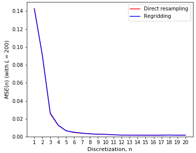
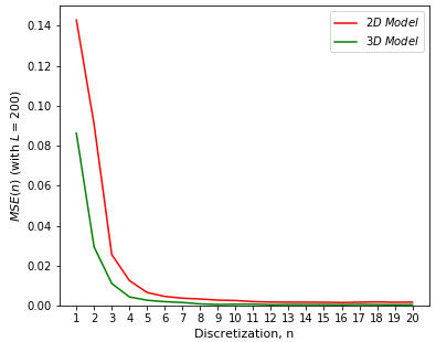
The number of recommended discretization points for flow-based upscaling remains the same as for a scalar property: \(5\) by \(5\) for 2-D and \(4\) by \(4\) by \(4\) for 3-D.

Summary

Grid block discretization has practical application in many areas of geostatistical estimation and simulation. Geological models built with a reasonable discretization level yield accurate resource estimates and are best utilized for flow studies. To model a 2-D block, a \(5\) by \(5\) discretization is recommended as it provides a stable value with low error. For a 3-D block, a \(4\) by \(4\) by \(4\) discretization is recommended. Composite data may require adjustment of the discretization number in the direction of drilling to the block size divided by the composite length.

References