Learning Objectives

• Understand the importance of high resolution data spacing models.
• Choose between constant number and constant volume calculations for 2D and 3D cases.
• Appreciate complex sampling configurations.

Introduction

Data spacing is the average distance between drill hole data within a volume. Although data spacing is often linked to regularly sampled and equally spaced drill holes, it can be calculated for any drilling configuration (Cabral Pinto, 2016; Wilde, 2010).

The calculation of data spacing is straightforward when the drill holes are equally spaced and drilled perpendicular to the plane of greatest continuity. In the presence of complex or irregular drilling, the data spacing must be calculated locally. Our recommendation is to calculate the data spacing for the same block model resolution as used in resource estimation.

Data spacing has been used as a geometric criterion for classification, as a measure of data availability, and to assess new sampling schemes. This lesson focuses on data spacing calculation where the spacing must be inferred from limited, regularly or irregularly spaced drilling. This lesson does not discuss optimal placement of infill drilling.

Concept

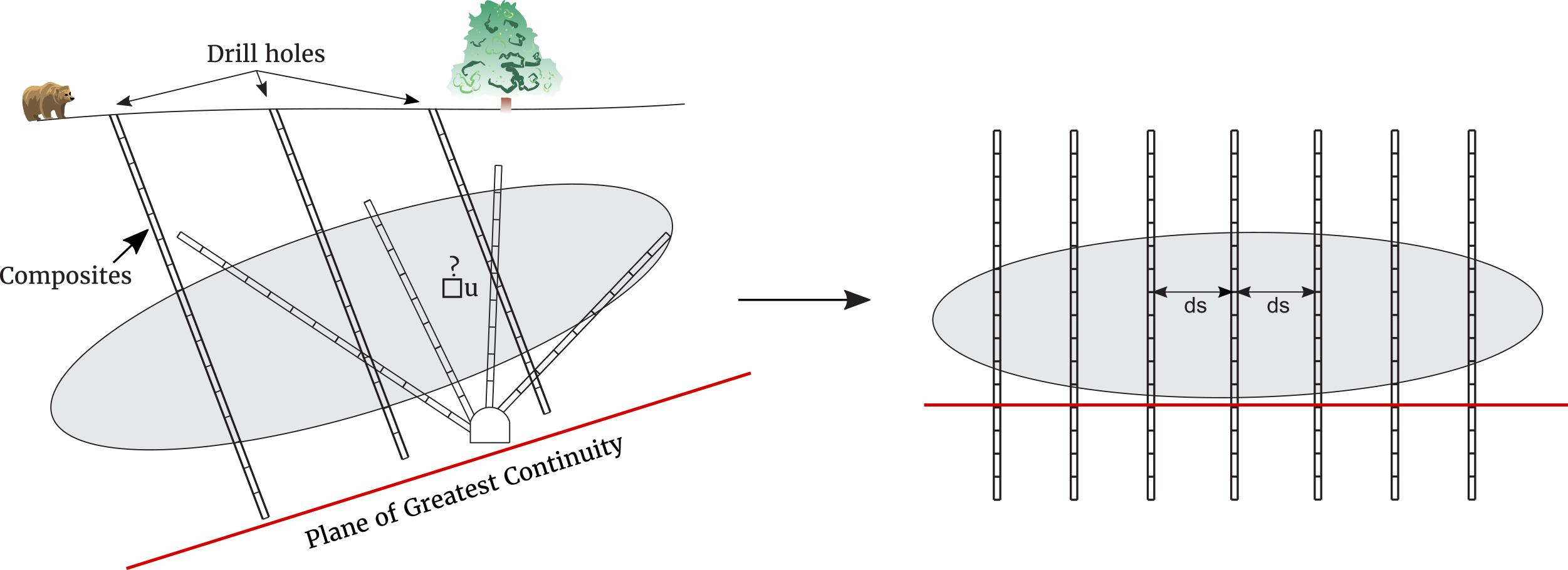
Considering the observed data density in a particular volume, we define “data spacing” as the equivalent square spacing for drill holes drilled perpendicular to the plane of greatest continuity. The calculation of the data spacing accounts for the composite length, irregular drilling directions, and the orientation of the plane of continuity. Our definition as the equivalent square drill hole spacing could be modified to a specific rectangular spacing if there is strong anisotropy in the plane of greatest continuity. The key idea of calculating the data spacing will be to either consider a constant number of data and find the corresponding volume or consider a constant volume and find the corresponding number of data. The figure below illustrates data spacing.

Calculation

When drill holes are aligned in the same direction, e.g., vertically, and fully intersect the zone of interest, the calculation of the data spacing (ds) is simplified to a 2D case. The data spacing could be calculated by either fixing the number of samples to search for n, and calculating the area A(u) to find them; or by fixing A and calculating n(u). Searching for a fixed number of data appears to be the most robust.

When searching for data, a circle is used to calculate the area represented by the fixed number of data. The radius used in the calculation of the area is the average distance of the last data to search r_n(u) and the next nearest data r_n+1(u). Additional practical details including the number of drill holes will be discussed below.

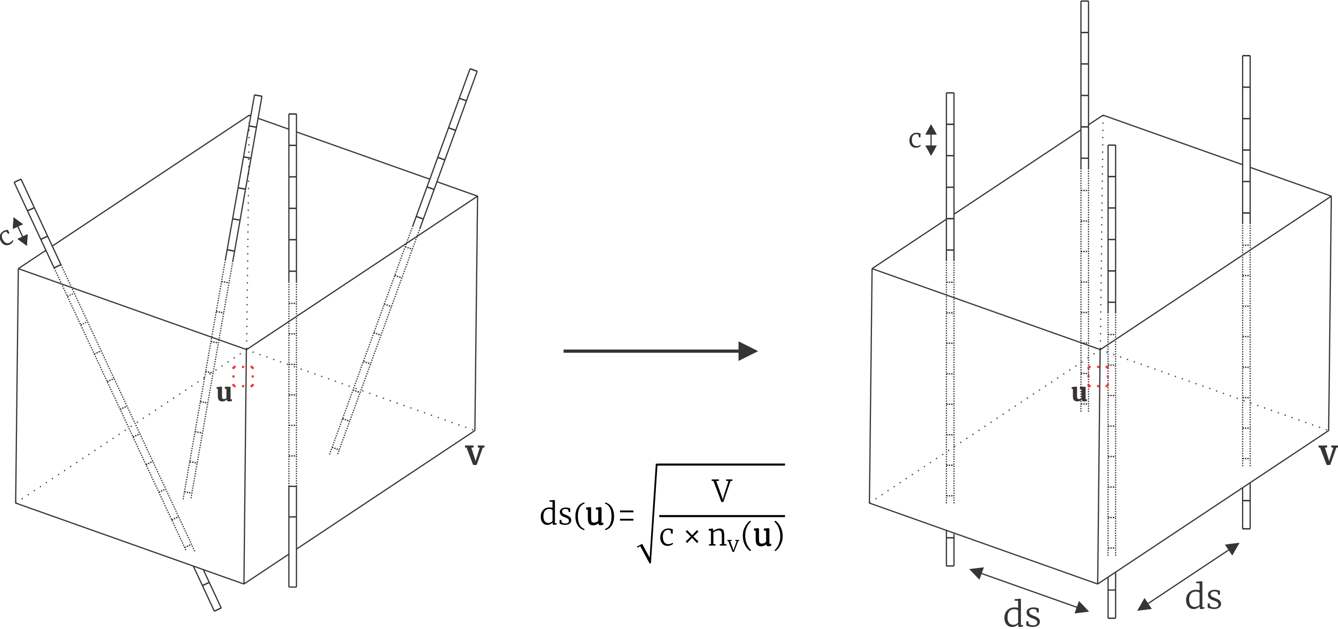
The calculation of the data spacing for 3D cases are often set up to consider a constant volume V, the composite length c, and the number of samples n(u) falling inside the volume. The volume could be an ellipsoid or a rectangular parallelepiped. The figure below shows a cube. The composite length is included to define the equivalent regular drill hole spacing. The data spacing is taken as the square spacing perpendicular to the plane of continuity that would give the same number of samples, n(u), as actually found. Practice has shown that using a volume 2 to 3 times the data spacing leads to reasonably stable results.

A Note on Data Density

Data density measures the number of data inside a reference volume. Data density is high if many data fall within a small volume and low if a large volume contains few data. Data density is an alternative to data spacing. For example, the number of drill holes per section is sometimes used in oil sands projects.

Practical Considerations

Some practical considerations on data spacing involve parameter selection and limitation of the area and volume.

Fixed Parameters

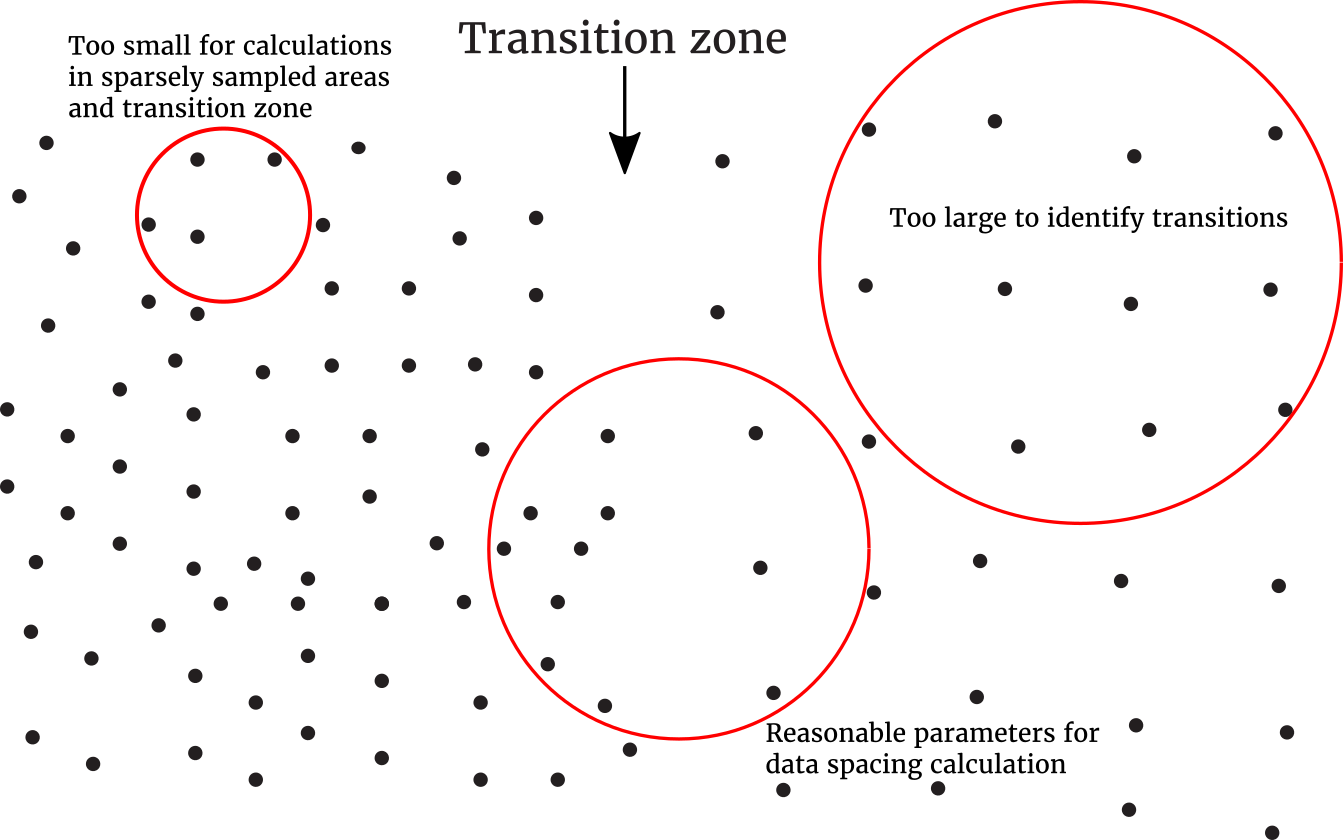
When choosing the parameters for data spacing calculation, the local neighbourhood must be large enough for stable estimates and to avoid artefacts near individual drill holes. The neighbourhood must be small enough to precisely identify transitions between areas of different spacing.

There is no theoretically correct number of samples. The result should appear reasonable and free of visual artefacts. The neighbourhood must be large enough to calculate the data spacing in sparsely sampled areas. For this reason the ideal search for data spacing may not coincide with the optimal kriging search ellipsoid.

Multiple Parameters

The number of data in 2D calculation and the volume in 3D calculation are parameters that must be chosen. In practice, the calculation of the data spacing with a single parameter, a fixed n or V, tends to be noisy for a few number of data or too small volume, and over smooth and locally less accurate for a great amount of data or too large volume. One approach is to consider multiple n and V values at each location and take the average of the resulting data spacing values (Silva & Boisvert, 2014). Practice has shown that the average of the values using n between 4 to 10 works well.

Depth and Aerial Limits

The data spacing could be used to clip a resulting estimated model. Blocks considered to be too far away from the data can be reset as unestimated. Moreover, the data spacing could be used to classify the blocks into measured, indicated and inferred resources. Extrapolation of the data spacing at depth and aerially beyond the data may be undesirable.

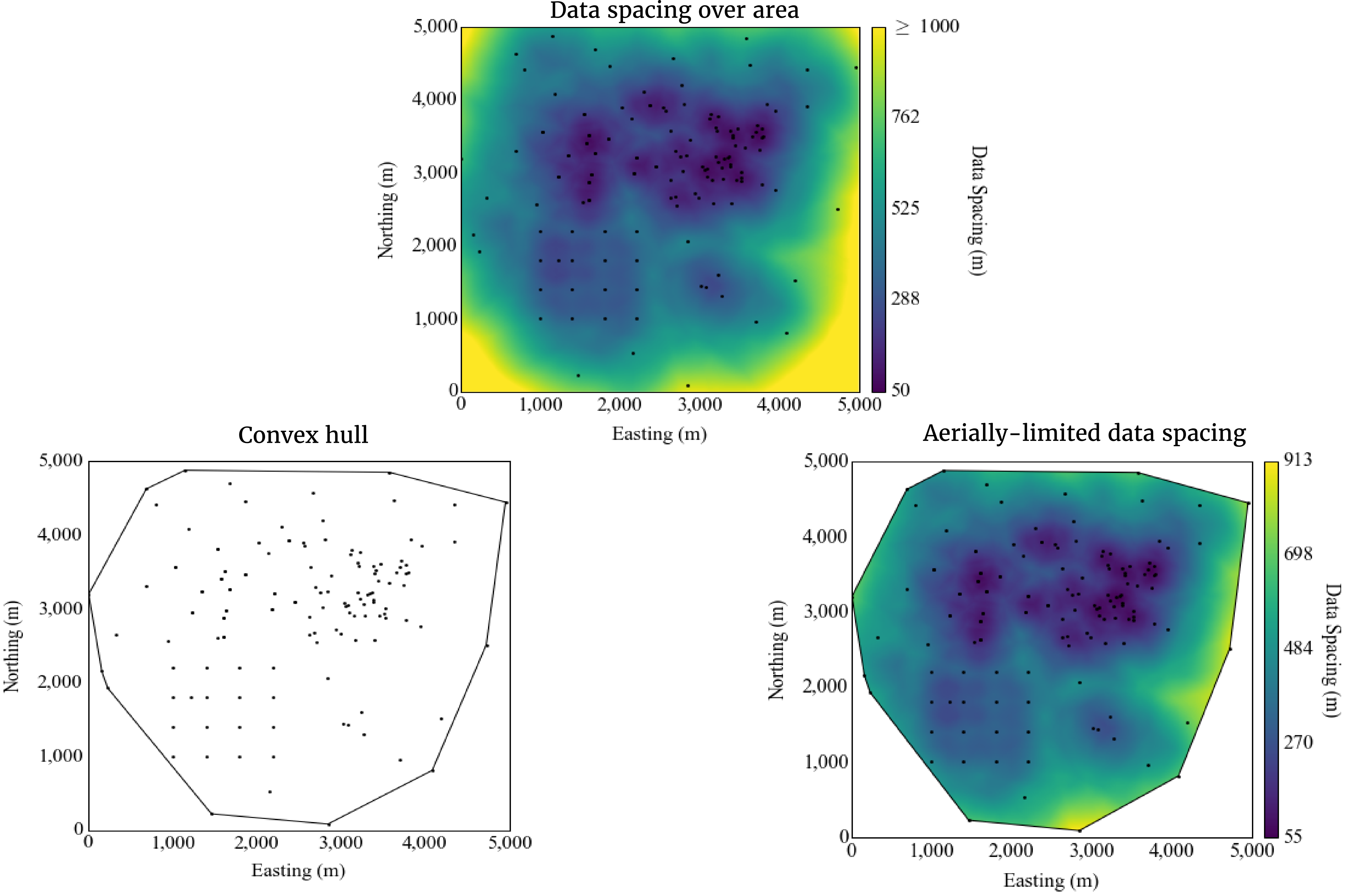
In some cases the depth of data spacing calculation is limited to the depth reached by nearby drill holes (Wilde & Deutsch, 2011). In addition to depth limits, aerial limits can be calculated using a convex hull. The data spacing calculation could be limited to locations within the convex hull. The decision to extrapolate or not would be made on a case-by-case basis depending on understanding of the geological continuity.

Summary

A high resolution data spacing model has many applications. The calculations are relatively simple, although care must be taken when choosing the parameters. Best practices involve fixing n and calculate A(u) in 2D, and fixing V and calculating n(u) in 3D cases. When choosing n or V, they should be small enough for local precision and large enough for a smooth, but not over smooth, data spacing calculation.

The idea behind data spacing is to calculate the equivalent regular drill hole spacing that would give the same amount of data. The results should be precise yet free of artefacts.

References