Learning Objectives

• Review why the variogram of original units is required.
• Motivate the calculation of the variogram of normal scores.
• Understand how a variogram of normal scores is transformed to original units.

Introduction

Establishing a reliable variogram for each regionalized variable is an important step in a geostatistical study. The variogram of the regionalized variable in original units is required for minimum error variance estimates and for average variogram values. The experimental variogram of the data in original units is often unstable and noisy due to (1) a highly skewed distribution with extreme values used differently in each lag, and (2) preferential sampling in high valued areas combined with the proportional effect leading to the experimental variogram at small distance lags being particularly unstable, that is, showing less structure.

The correlogram partially addresses these sources of a noisy variogram, but it is theoretically incorrect and fails to correctly represent zonal anisotropy and trends. The pairwise relative variogram is remarkably stable, but is also theoretically incorrect. Variograms of indicator, logarithm or normal scores transforms are also theoretically inconsistent with the correct original units variogram. These robust alternatives to the variogram provide insight into the spatial structure of a variable, but should not be used for kriging the variable in original units or for calculating the expected variance within blocks.

A useful and theoretically correct approach is to start by calculating the variogram on the normal score transform of the variable. The variogram of normal scores is used directly in Gaussian techniques and can also be transformed to correctly represent the variogram of original units. The transformation could be done either for each lag or for the variogram model of the normal scores. The transformed variogram would be fit by commonly used variogram structures to facilitate the use in kriging and average variogram programs.

The transformation of a normal scores variogram to original units could be done with Hermite polynomials or by a straightforward Monte Carlo Simulation (MCS) approach (Vann & Sans, 1995; Wilde & Deutsch, 2006). The results are exactly the same (Wilde & Deutsch, 2007). The approach with Hermite polynomials was implemented by Wilde for testing (Wilde & Deutsch, 2007). It has been available in the geovariances software (http://geovariances.com) for many years. The MCS approach is described here. Some details of the normal scores transformation and variogram calculation are provided. The variogram transformation is described, then some examples are presented.

Normal Scores Transform

The univariate normal scores transform is well established. A representative non-parametric distribution of the regionalized variable is required \(F(z)\). Declustering or calibration with a secondary variable may be required to make \(F(z)\) as representative as possible of the entire stationary domain. The data \(z_i,i=1,\ldots,n\) may have constant values at detection limit or due to the number of decimal places used in the database. These spikes of constant values must be despiked. A combination of local average and random despiking could be considered to avoid a bias in the experimental variogram. The despiked data \(z_i,i=1,\ldots,n\) are then transformed to normal scores by matching quantiles to the Gaussian distribution: \(y_i=G^{-1}(F(z_i)),i=1,\ldots,n\) where \(G^{-1}( \cdot )\) is the inverse of the standard normal cumulative distribution.

The equal weighted variance of the normal score data \(y_i,i=1,\ldots,n\) will not necessarily be one if declustering is considered. The experimental normal score variogram should be standardized by the equal weighted variance of the normal scores. A comparative study (not documented here) considering this approach, not standardizing the variogram and normal score transformation without the declustering weights showed that this approach led to results closer to the underlying true variogram.

Experimental variograms calculated on the normal scores are often more stable than those calculated on the original units. Extreme values are mitigated and an apparent lack of structure due to clustering and the proportional effect is also mitigated. The experimental variogram may still be unreliable in presence of few data or widely spaced data relative to the variogram range. Variograms from geologic analogues may need to be considered. If the experimental variogram of the normal scores is reasonable then it can be transformed to represent the original units.

Transformation of the Variogram of Normal Scores

The variogram for each lag of the experimental normal scores variogram is transformed one at a time. Consider one experimental normal scores variogram value \(\hat{\gamma_Y}\). Assuming that the normal score values are second order stationary the corresponding correlation coefficient is \(\rho=1-\hat{\gamma_Y}\). Many pairs are sampled from a bivariate Gaussian distribution with standard marginal distributions and a correlation of \(\rho\).

Start with pairs sampled independently from a standard normal distribution: \(y_{s1}^l, y_{s2}^l, l=1,\ldots,L\). These independent pairs are correlated with a correlation of \(\rho\) are given by \(y_1^l = y_{s1}^l\) and \(y_2^l = y_{s1}^l \cdot \rho + y_{s2}^l \cdot \sqrt{1-\rho^2}, l=1,\ldots,L\). This is equivalent to drawing pairs from the bivariate standard normal distribution. These paired values are back transformed to \(z_1^l=F^{-1}(G(y_1^l))\) and \(z_2^l=F^{-1}(G(y_2^l))\). The transformed original variogram for this lag is then calculated as:

\[ \hat{\gamma_Z} = \frac{1}{L} \sum_{l=1}^{L} (z_1^l-z_2^l)^2 \]

Considering many pairs (\(L=10^5\)) leads to a stable variogram value in original units \(\hat{\gamma_Z}\) that corresponds to the calculated experimental variogram in normal score units \(\hat{\gamma_Y}\). The TransformYZ program (http://ccgalberta.com/) implements this simple approach. In practice, extreme values in the back transform to \(z_1^l\) and \(z_2^l\) may be capped to make the variogram even more stable.

The transformed variogram is more reliable than a variogram calculated directly on the original units data because (1) the assumption of second order stationarity is considered in the transformation, that is, the marginal distributions for each lag are assumed stationary, (2) the skewed distribution and extreme values are considered equally in all lags, and (3) the influence of extreme values could be further mitigated by capping the high values in the back transformation.

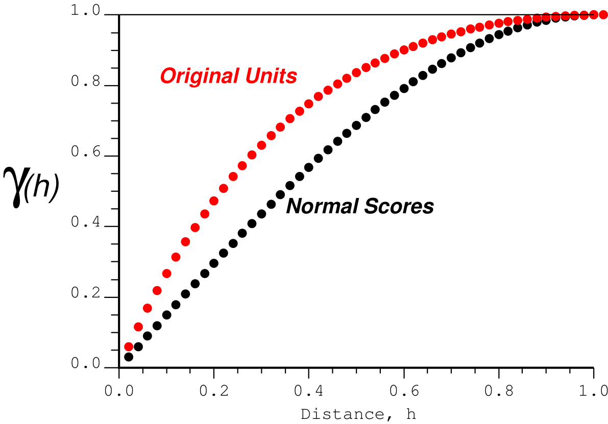
In the presence of a highly skewed distribution, the variogram of original units will show less structure than the variogram of normal scores. Consider a second order stationary regionalized variable that follows a lognormal distribution with a coefficient of variation of 2. An analytical relationship between the variograms is known and can be used to test any software implementation. The figure below shows the results. Note the significant difference between the variograms.

The analytical relationship for the standardized original units variogram for a lognormal distribution is given by:

\[ \gamma_Z = 1 - \frac{(1+CV^2)^{1-\gamma_Y} -1}{CV^2} \]

where CV is the coefficient of variation.

Examples

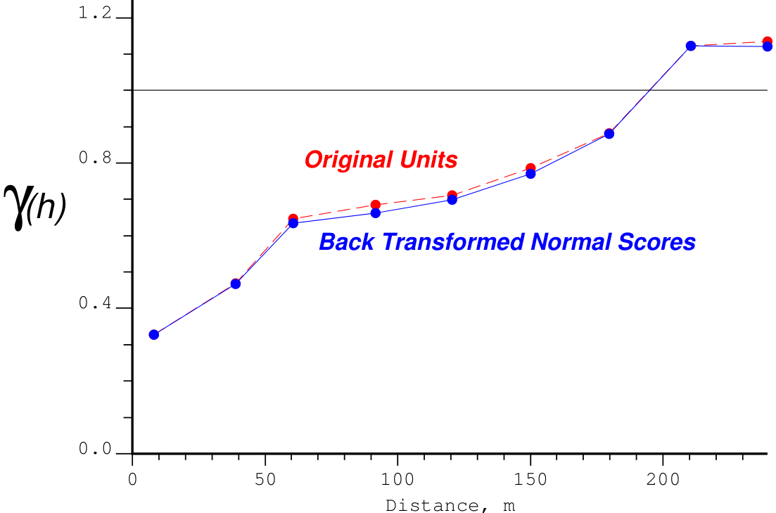
The first example is from gold grades in the plane of an epithermal vein. The experimental variogram of original units (red points and dashed line) are virtually identical to the transformed normal scores variogram (blue points and solid line). This is common when there is no unequal influence due to outliers and no clustering and proportional effect.

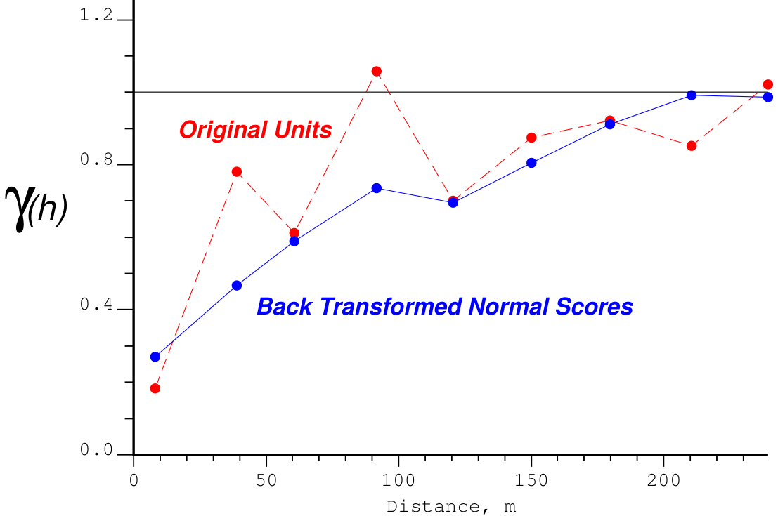
The second example is from copper grades in a skarn deposit. The experimental variogram of original units is quite noisy (red points and line). The transformed normal scores variogram (blue points and solid line) is more stable and would be easier to model. Outliers in the original data are causing the noise in the original units variogram.

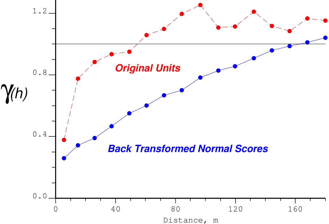
The third example is from gold grades in a porphyry deposit. The experimental variogram of original units (red points and line) is reasonably stable, but shows relatively little structure because of the proportional effect and clustering. The transformed normal scores variogram (blue points and solid line) shows very clear structure. The large discrepancy in this case is due to strong clustering and the proportional effect.

The last two examples show significant differences. They were chosen for this reason. In many cases, like the first example, the results will be very close. The authors have not encountered a case where the normal score variogram transformed to original units is worse. The theory is simple and robust.

Discussion

The procedure advocated here is to (1) inspect the data looking for extreme values, clustering and the proportional effect - as an explanation for why the straightforward calculation of the original units variogram may be unreliable, (2) calculate the variogram of original units as a check, (3) normal score transform the declustered and despiked data, (4) compute the standardized variogram on the normal scores, (5) transform the normal scores variogram to original units, and (6) compare the results and proceed with the normal scores variogram for Gaussian techniques and the deemed representative original units variogram for kriging and expected variance calculations. Many of these steps could be automated in software.

There may be doubt in cases like the third example shown above. The variograms are very different and the fact that the back transformed original units variogram shows more structure does not necessarily make it correct. If outliers and clustering are the obvious explanation, then proceeding with the transformed variogram is reasonable. If doubt persists, then further checking such as jackknife validation, decimate the clustered data, and comparison with production sampling should be undertaken.

Summary

A variogram representing the original units of a regionalized variable is needed for kriging and calculating the expected variance within different block sizes. It would be an error to use a robust alternative to the variogram or the untransformed variogram of normal scores. The more robust normal scores variogram can be calculated and then transformed to represent original units. The normal scores variogram could also be used directly for prediction of local uncertainty and simulation. The normal scores and original units variograms could be quite different from each other, yet consistent.

References