Learning Objectives

• Understand linear decorrelation transforms that are extensions of principal component analysis (PCA), including data sphereing and min/max autocorrelation factors (MAF).
• Review essential sphereing and MAF theory, highlighting the reasons that they may outperform PCA within the context of geostatistical modeling.
• Interpret sphereing and MAF results to consolidate understanding of the techniques.

Introduction

This lesson describes linear decorrelation transforms that are direct extensions of principal component analysis (PCA). The transforms are presented in the context of modeling multiple geological variables with a decorrelation workflow:

1. A transform is used to decorrelate the variables
2. Transformed variables are modeled under the assumption of independence
3. The back-transform restores the original correlation to the modeled variables

Most linear decorrelation transforms also facilitate dimension reduction, where a subset of the variables are modeled, before the back-transforms provide models of all variables. The transforms that will be introduced in this lesson, data sphereing and min/max autocorrelation factors (MAF), may outperform PCA within this framework.

This lesson begins with a brief review of PCA, although readers are encouraged to review the Principal Component Analysis lesson if unfamiliar with the technique and related concepts such as spectral decomposition and transform loadings. Sphereing and MAF are then introduced and demonstrated, before summarizing their key features.

Principal Component Analysis

Consider \(k\) variables \(Y_1,\ldots,Y_k\) that have been standardized to have a mean of zero (required for linear rotations) and variance of one (recommended for linear rotations). Conditioning data is given as the matrix \(\mathbf{Y}: y_{\alpha, i}, \alpha=1,\ldots,n, i=1,\ldots,k\), where \(n\) is the number of samples. The primary input to PCA is the covariance matrix:
\[ \boldsymbol{\Sigma}: C_{i,j}=\frac{1}{n} \sum_{\alpha=1}^n y_{\alpha,i} \cdot y_{\alpha,j}, \text{ for } i,j=1,\ldots,k\]

Diagonal entries \(C_{i,i}\) are the variance of each \(Y_i\). Off-diagonal entries \(C_{i,j}, i \ne j\) are the covariance between \(Y_i\) and \(Y_j\). These covariances are also correlations since each \(Y_i\) has a variance of one. The first step of PCA performs spectral decomposition of \(\boldsymbol{\Sigma}_Y\), yielding the orthogonal eigenvector matrix \(\mathbf{V}_Y:v_{i,j},i,j=1,\ldots,k\) and the diagonal eigenvalue matrix \(\mathbf{D}_Y:d_{i,i},i=1,\ldots,k\): \[\boldsymbol{\Sigma}_Y = \mathbf{V}_Y\mathbf{D}_Y\mathbf{V}_Y^T\]

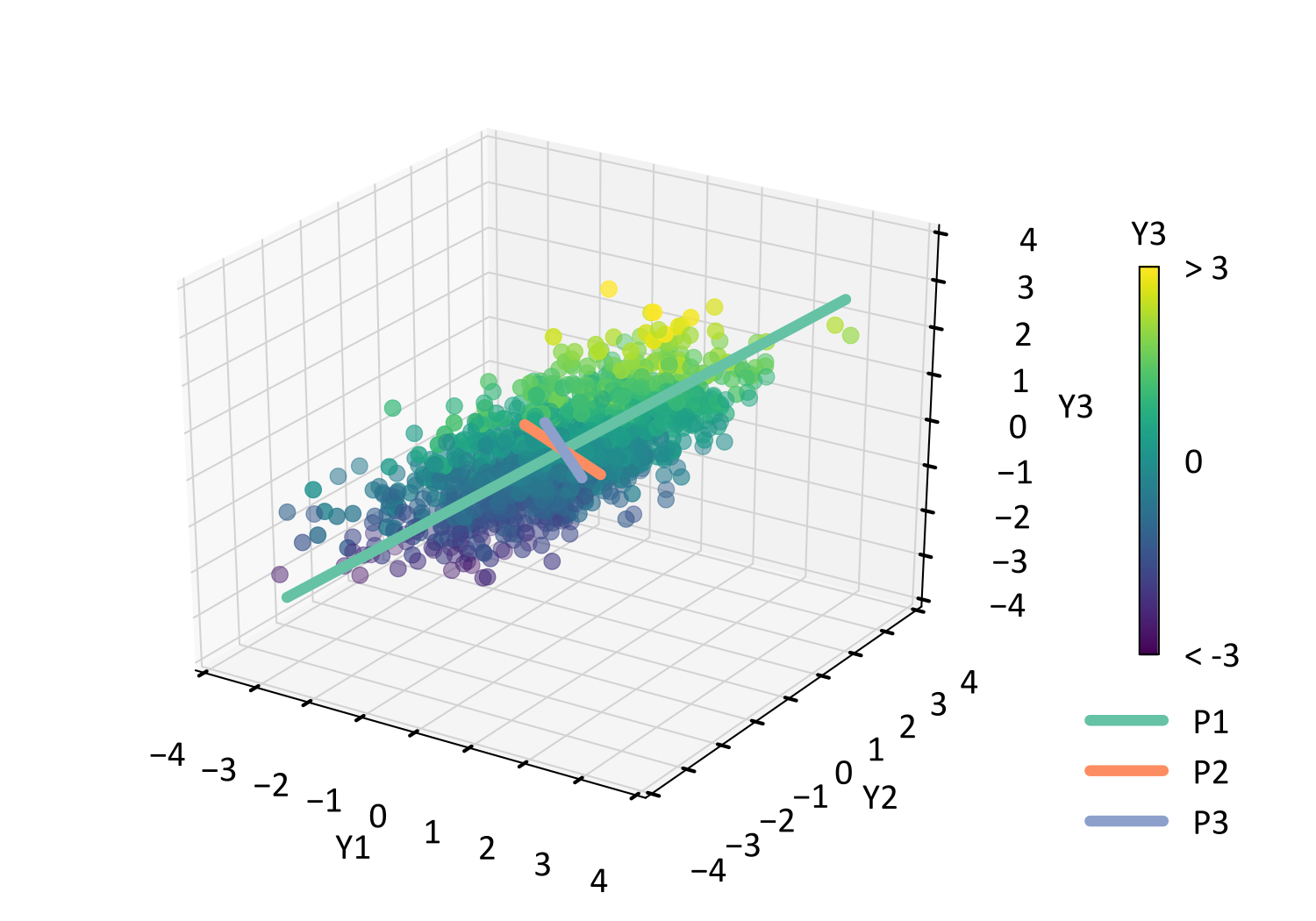
This is demonstrated using a small \(k=3\) example, where a scatter plot of the original \(Y_1,\ldots,Y_3\) data is overlain with vectors, whose orientation and length represent each eigenvector column and diagonal eigenvalue entry respectively.

The PCA transform is then performed through the matrix multiplication of \(\mathbf{Y}\) and \(\mathbf{V}_Y\): \[\mathbf{P}= \mathbf{YV}_Y\]

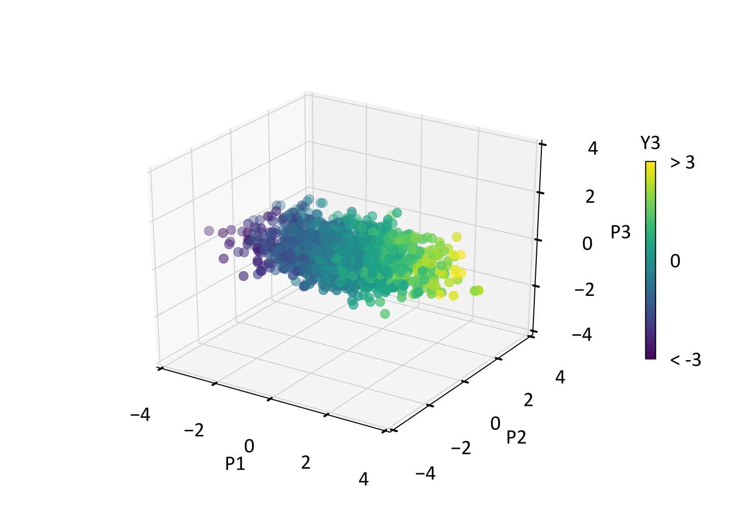
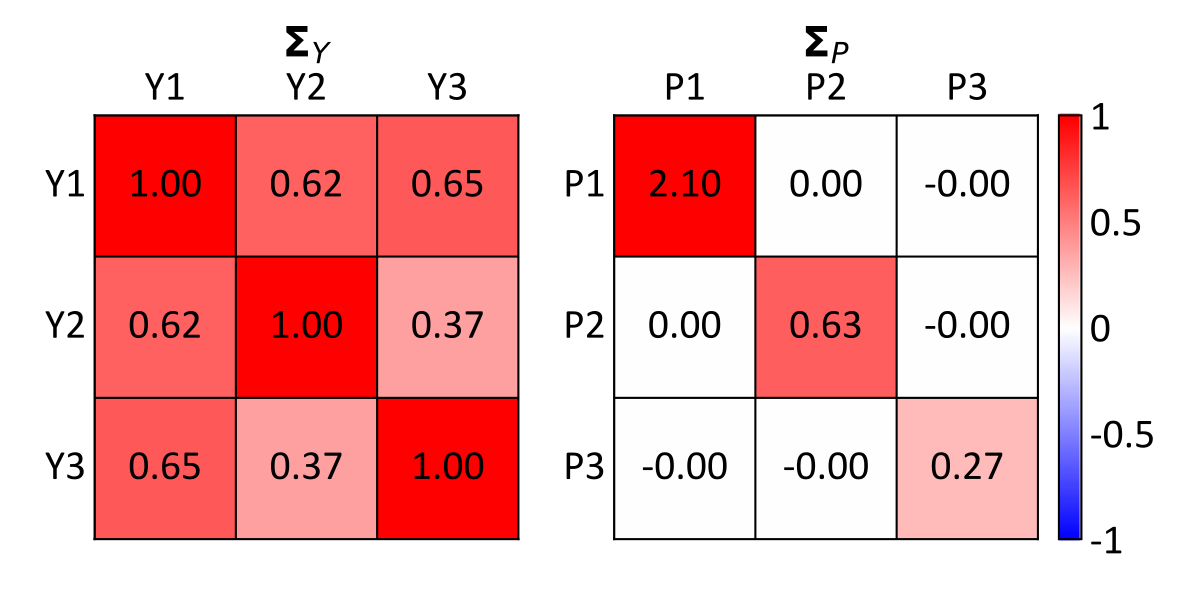
This rotates the multivariate data so that the resultant principal components in \(\mathbf{P}\) are uncorrelated, where off-diagonal entries of its correlation matrix \(\boldsymbol{\Sigma}_P\) are zero. Direct entries of \(\boldsymbol{\Sigma}_P\) are the variance of the principal components, which correspond with the eigenvalues in \(\mathbf{D}_Y\). The below scatterplot displays the transformed data \(P_1,\ldots,P_3\), where \(Y_1,\ldots,Y_3\) from the previous scatterplot are rotated to be uncorrelated.

Data Sphereing

Data sphereing is a class of rotations that are close extensions of PCA, yielding variables that in addition to being uncorrelated, also have a variance of one. The combination of these properties yields an identity covariance matrix. Also known as data whitening, two available forms of sphereing are referred to here as dimension reduction sphereing (DRS) (Friedman, 1987) and spectral decomposition sphereing (SDS) (Fukunaga, 1972; Hwang, Lay, & Lippman, 1994).

DRS Transform

DRS is the simpler of the two sphereing transforms and is given as: \[\mathbf{W}=\mathbf{Y}\mathbf{S}^{-1/2}, \text{ where } \mathbf{S}^{-1/2} = \mathbf{V}_Y\mathbf{D}_Y^{-1/2}\]

The multiplication of \(\mathbf{V}_Y\) rotates the variables to an orthogonal axis (PCA), before \(\mathbf{D}_Y^{-1/2}\) transforms them to have a variance of one. A more intuitive formulation of this transform may be \(\mathbf{W} = \mathbf{P}\mathbf{D}_Y^{-1/2}\), where each principal component \(P_i\) is divided by its standard deviation \(d_{i,i}^{1/2}\). The \(\mathbf{S}^{-1/2}\) term is commonly referred to as the sphereing matrix since it provides the transform. Multiplying \(\mathbf{W}\) by the inverse of the sphereing matrix provides the back-transform.

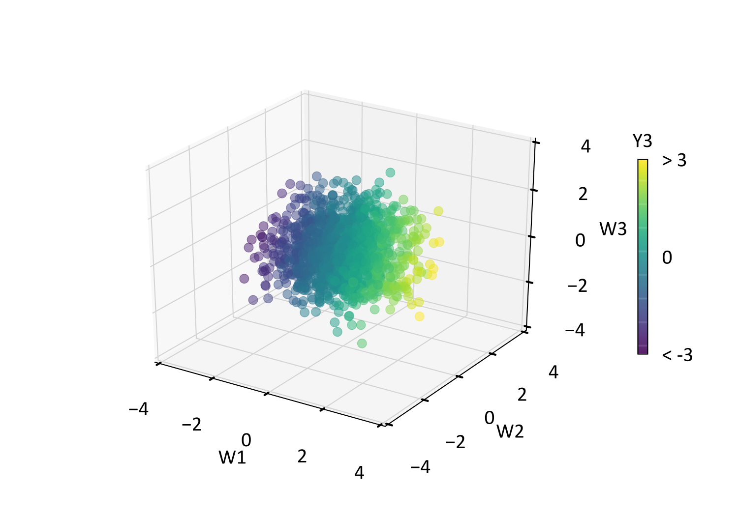
The difference between PCA and DRS is visually apparent in their respective scatterplots, where the differing variability of \(P_1,\ldots,P_3\) above is made uniform in \(W_1,\ldots,W_3\) below. This is confirmed by comparing diagonal entries of the covariance matrices \(\boldsymbol{\Sigma}_P\) and \(\boldsymbol{\Sigma}_W\) below, where the latter has the expected identity values. Using the \(Y_3\) scatter coloring for reference, note that the rotation is preserved between PCA and DRS.

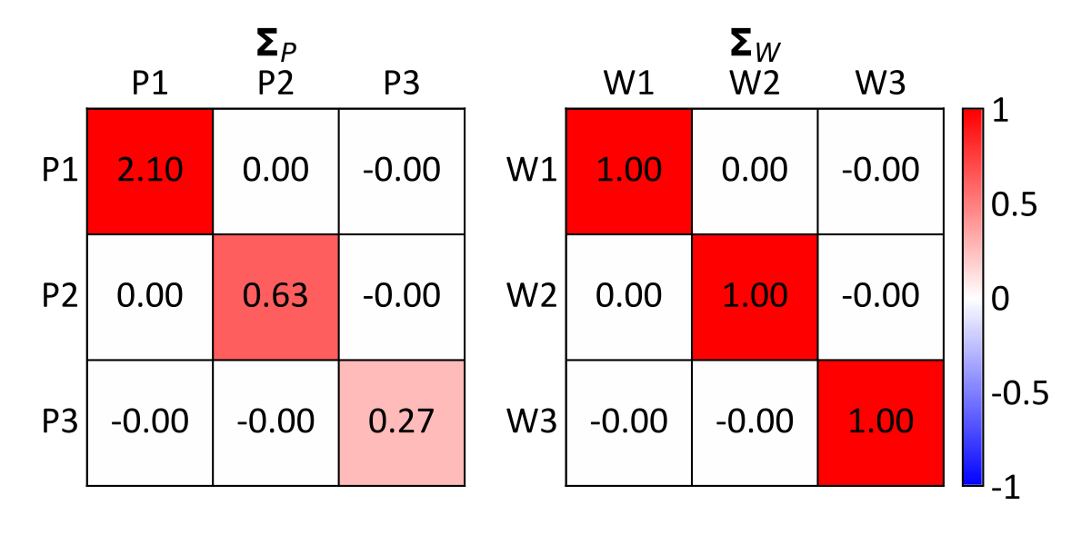
Although diagonal entries of \(\boldsymbol{\Sigma}_W\) do not correspond with the eigenvalues in \(\mathbf{D}_Y\) (as is the case with \(\boldsymbol{\Sigma}_P\)), the variability that each \(W_i\) explains about \(Y_1,\ldots,Y_k\) corresponds with the principal components \(P_1,\ldots,P_k\), since the loading \(\rho'\) is identical for PCA and DRS. More formally, \(\rho'(Y_i ,P_j ) = \rho (Y_i ,P_j ) \cdot \sigma_i = \rho'(Y_i ,W_j )\) for \(i,j=1,\ldots,k\), where \(\sigma_i\) is the standard deviation of \(Y_i\) (one since standardized), and \(\rho (Y_i ,P_j)\) is the correlation between \(Y_i\) and \(P_j\). DRS may therefore be useful if the properties of the PCA transform are required, while simultaneously benefiting from standardized variance in terms of interpretability and modeling convenience.

SDS Transform

Maximizing the multivariate variability that each descending PCA and DRS variable explains is useful for dimension reduction, but promotes mixing of the original variables in transformed space. More specifically, attempting to load \(Y_i,i=1,\ldots,k\) onto the first few \(P_i\) or \(W_i\) variables effectively increases their mixing in transformed space. This decreases the likelihood that the distinct characteristics of each variable \(Y_i\) are recovered following geostatistical simulation and back-transformation, motivating the SDS transform: \[\mathbf{X}=\mathbf{Y}\mathbf{S}^{-1/2}, \text{ where } \mathbf{S}^{-1/2} = \mathbf{V}_Y\mathbf{D}_Y^{-1/2}\mathbf{V}_Y^T\]

The difference between the two sphereing methods is the additional multiplication by \(\mathbf{V}^T\), which projects the orthogonal variables back onto the basis of the original variables. This aligns it with the form of the underlying spectral decomposition equation \(\boldsymbol{\Sigma}_Y = \mathbf{V}_Y\mathbf{D}_Y\mathbf{V}_Y^T\), explaining the derivation of its name. The rotation is performed in a manner that maximizes the absolute value of the loading \(\rho'(Y_i ,X_j )\) for \(i=j\), while minimizing the absolute value of \(\rho'(Y_i ,X_j )\) for \(i \neq j\). Thus, variables are made uncorrelated with minimal rotation, or minimal mixing in transformed space.

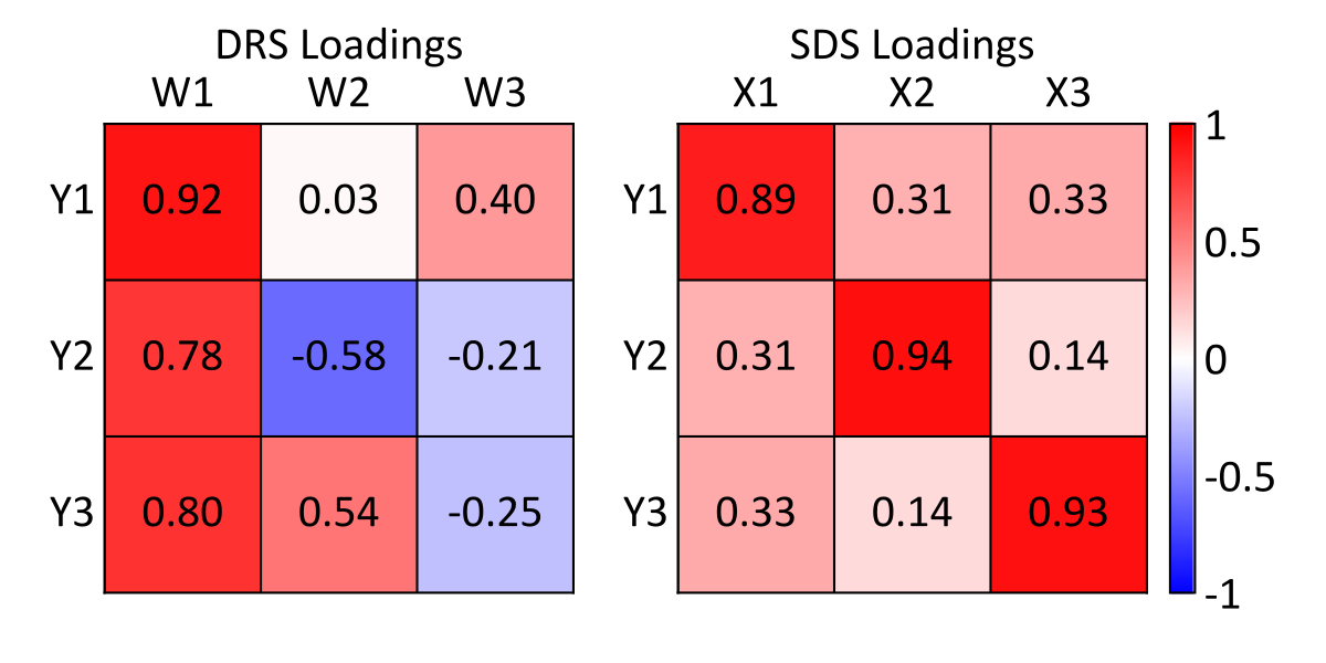
Consider that the \(Y_3\) coloring aligns more closely with the \(P_1\) and \(W_1\) axes for the PCA and DRS scatter above. This is expected since the first principal component explains the majority of variability, including \(Y_3\) variability. This is corroborated by the DRS loading matrix (below), where the largest loading of \(Y_3\) occurs on \(W_1\). Conversely, \(Y_3\) coloring closely aligns with the \(X_3\) axis in the SDS scatter below, while the SDS loading matrix shows that \(Y_3\) is loaded almost entirely on \(X_3\).

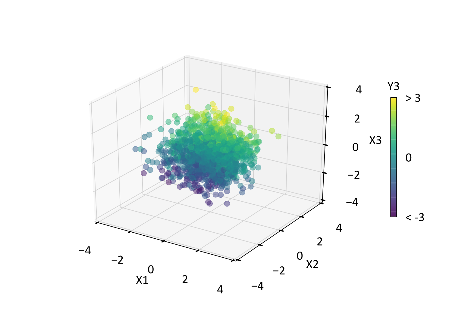
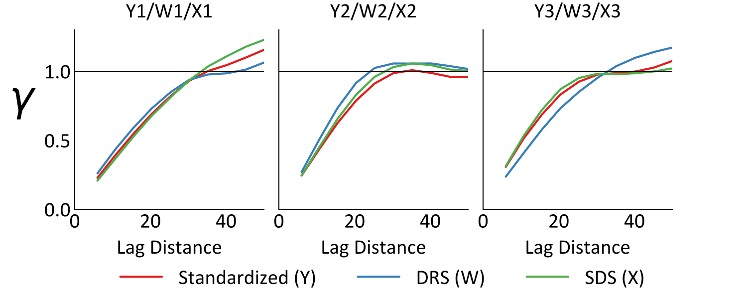
Variograms of the original and transformed variables confirm the expected behavior of the differing loadings, where the SDS variograms closely align with the original variograms. Conversely, the spatial structure of the original variables are heavily mixed in the DRS variables, yielding variograms that differ from the original variables. Simulated realizations of the SDS variables would therefore be expected to reliably reproduce the original variograms following back-transform. Simulated realizations of the DRS variables may reproduce the original variograms following back-transformation, though practice has shown that this is less reliable than the SDS approach.

Min/Max Autocorrelation Factors

MAF was introduced by (Switzer & Green, 1984) in the field of spatial remote sensing and popularized in geostatistics by (Desbarats & Dimitrakopoulos, 2000). Before motivating the technique, let the SDS transformed data be \(\mathbf{X}: x_i(\mathbf{u}_{\alpha}), \alpha=1,\ldots,n, i=1,\ldots,k\), where \(\mathbf{u}_{\alpha}\) is a coordinate vector. Spatial locations are separated by a lag vector \(\mathbf{h}\), which has a distance of \(h\). Spatial structure of the SDS variables is calculated using with the variogram matrix: \[\boldsymbol{\Gamma}_X: \gamma_{i,j}(\mathbf{h})=\frac{1}{2n(\mathbf{h})} \sum_{\alpha=1}^{n(\mathbf{h})} \big( x_i(\mathbf{u}_{\alpha}) - x_i(\mathbf{u}_{\alpha}+\mathbf{h}) \big) \big( x_j(\mathbf{u}_{\alpha}) - x_j(\mathbf{u}_{\alpha}+\mathbf{h}) \big) \\ \text{ for } i,j=1,\ldots,k\]

where there are \(n(\mathbf{h})\) samples separated by \(\mathbf{h}\). Note that \(\boldsymbol{\Gamma}_X\) is more strictly referred to as the semivariogram, though it is common practice in geostatistics to refer to it as the variogram. A diagonal value \(\gamma_{i,i}(\mathbf{h})\) is the variogram of \(X_i\), which relates to its autocorrelation \(C_{i,i}(\mathbf{h})\) according to \(\gamma_{i,i}(\mathbf{h}) = 1 - C_{i,i}(\mathbf{h})\). An off-diagonal value \(\gamma_{i,j}(\mathbf{h}),i \ne j\) is the cross-variogram between \(X_i\) and \(X_j\), which relates to their cross-correlation \(C_{i,j}(\mathbf{h})\) according to \(\gamma_{i,j}(\mathbf{h}) = -C_{i,j}(\mathbf{h})\). This is based on applying the general relation \(\gamma_{i,j}(\mathbf{h})=C_{i,j}(0)-C_{i,j}(\mathbf{h})\), where the \(C_{i,j}(0)\) values are drawn from the identity covariance matrix \(\boldsymbol{\Sigma}_X\) in this case.

MAF Motivation

An implicit assumption of geostatistical modeling frameworks that utilize PCA or sphereing, is that in decorrelating the variables at zero lag, \(C_{i,j}(0)=0\), the variables are decorrelated at all lags, \(C_{i,j}(\mathbf{h})=0\) for all \(\mathbf{h}\). Consider cross-variograms for the presented example below, which are significantly reduced by sphereing, but not made zero.

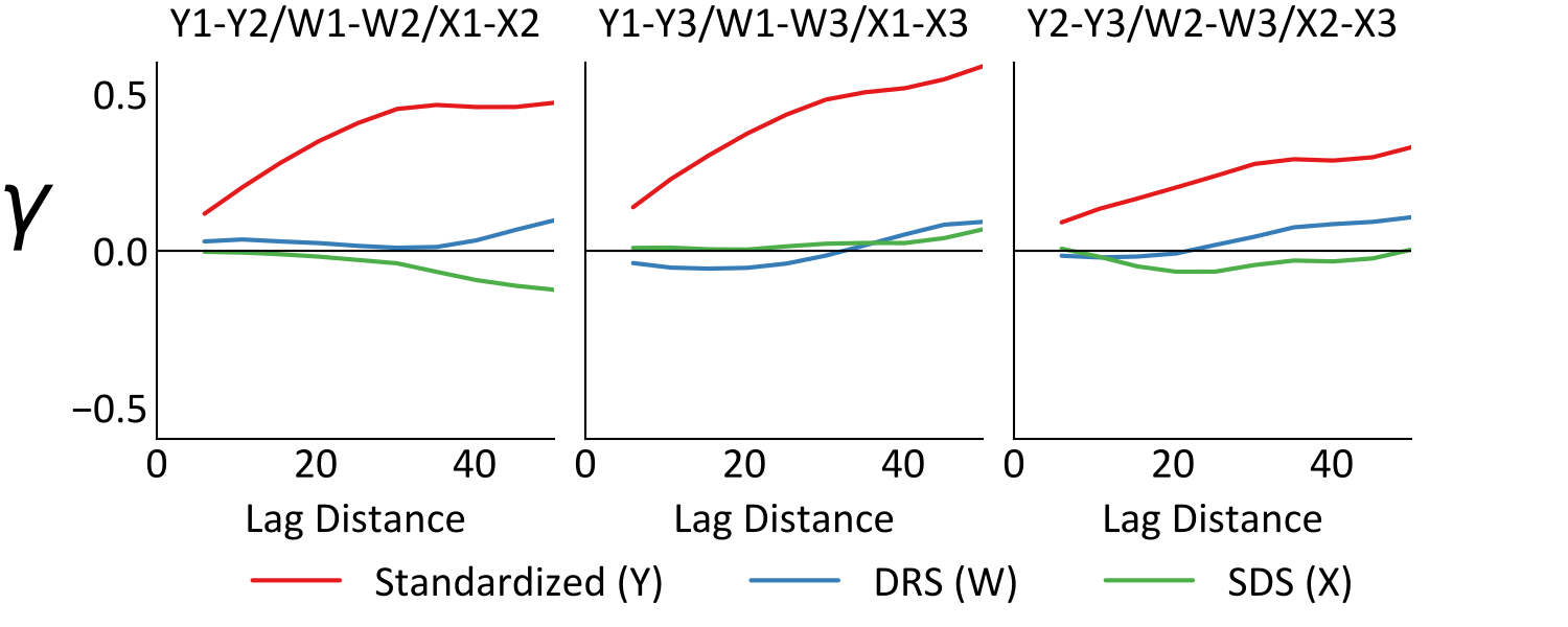
Independent simulation in the presence of significant cross-variogram values will lead to issues with the reproduction of the original variogram and cross-variograms, as well as other properties. This motivates MAF, which transforms variables to be uncorrelated at \(h=0\) and one \(h>0\) lag. If the spatial correlation can be described by a two-structure linear model of coregionalization (LMC) (Journel & Huijbregts, 1978), then the MAF transformed variables will be made uncorrelated for all \(\mathbf{h}\). This in turn, should lead to improved cross-correlation reproduction in simulated realizations. Even where the variables are not fully described by a two structure LMC, MAF has still been found to yield better cross-correlation reproduction than PCA (Barnett & Deutsch, 2012).

MAF Transform

The MAF workflow is summarized with four steps:

1. Perform spectral decomposition of the \(\mathbf{Y}\) covariance matrix \(\boldsymbol{\Sigma}_Y = \mathbf{V}_Y\mathbf{D}_Y\mathbf{V}_Y^T\)
2. Perform the DRS or SDS transform (SDS used here), \(\mathbf{X} = \mathbf{Z}\mathbf{V}_Y\mathbf{D}_Y^{-1/2}\mathbf{V}_Y^T\)
3. Perform spectral decomposition of the \(\mathbf{X}\) variogram matrix \(\boldsymbol{\Gamma}_X = \mathbf{V}_X\mathbf{D}_X\mathbf{V}_X^T\)
4. Perform the MAF transform, \(\mathbf{M} = \mathbf{X}\mathbf{V}_X\)

This two-step spectral decomposition and rotation yields multivariate data so that the resultant autocorrelation factors in \(\mathbf{M}\) are uncorrelated at \(h=0\) and the \(\mathbf{r}\) lag that was used for the calculation of \(\boldsymbol{\Gamma}_X\). The \(\mathbf{r}\) lag should have a distance \(r\) that is greater than zero. The MAF back-transform is given as \(\mathbf{Y}=\mathbf{M}\mathbf{A}^{-1}, \text{ where } \mathbf{A} = \mathbf{V}_Y\mathbf{D}_Y^{-1/2}\mathbf{V}_Y^T\mathbf{V}_X\).

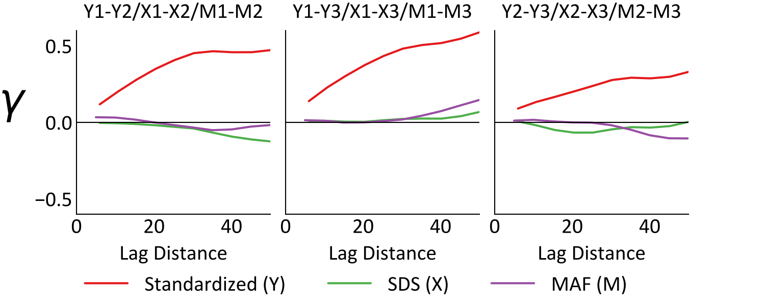
Scatterplots of the MAF data are displayed below, where the rotation is apparent based on \(Y_3\) coloring relative to the SDS scatterplot. The more obvious characteristic of the MAF transform, however, is seen when comparing its cross-variogram to that of the SDS and original data. The cross-correlation for MAF is generally less than that of SDS at short scale lags, and is made zero at the \(r=20\text{m}\) distance that is used for the calculation of \(\boldsymbol{\Gamma}_X\).

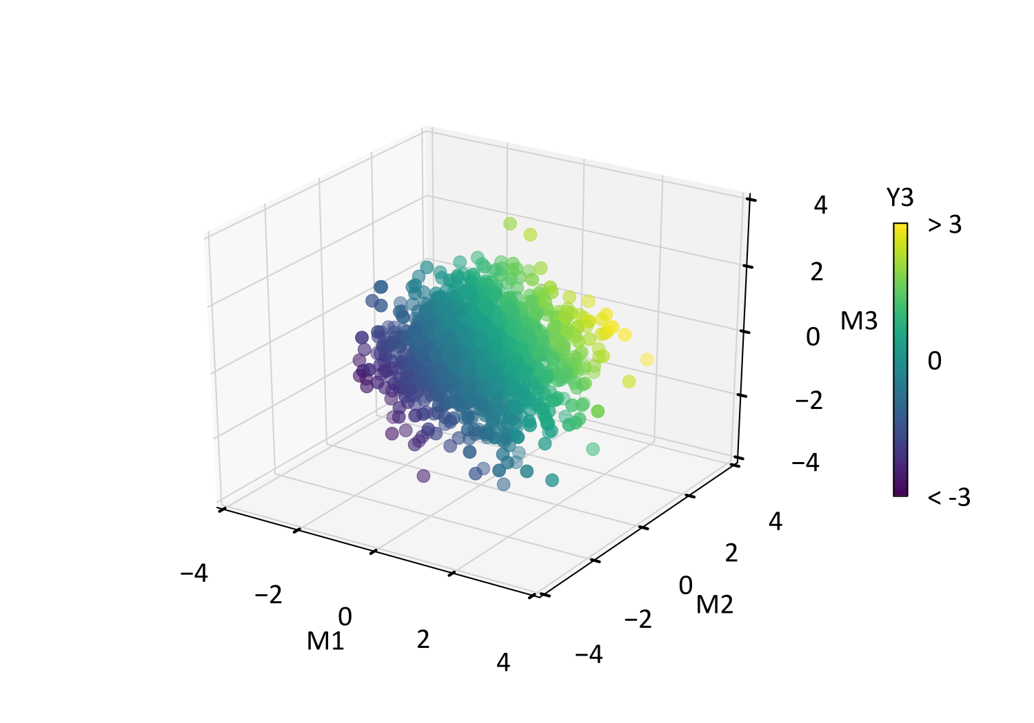
Selection of the \(\mathbf{r}\) lag is not straight forward. Iterative execution of MAF with varying \(\mathbf{r}\) is one option, before selecting the lag that provides the least cross-correlation overall. Consider that with variogram modeling, priority is often placed on the reproduction of short-scale features. Extending this concept, the use of a smaller \(\mathbf{r}\) will generally remove short scale cross-correlation, leading in turn to the reproduction of short scale cross-correlation following simulation and back-transformation. Readers using a web browser may use the following interactive figure, which displays the cross-variogram of the example \(\mathbf{M}\) data with varying \(r\) distances.

Cross-variogram of the MAF transformed data. Use the slider at the bottom to manipulate the decorrelation lag distance.

Dimension Reduction

As with PCA, MAF provides dimension reduction functionality that allows for less than the \(k\) variables to be simulated, before the back-transform provides realizations of all \(k\) original variables. Caution should be used, however, as the variability that is described by eigenvalues in \(\mathbf{D}_Y\) (PCA) and \(\mathbf{D}_X\) (MAF) is very different.

The diagonal entries of \(\mathbf{D}_Y\) are rank ordered according to the variability that each \(Y_i\) principal component explains about the multivariate system, while also corresponding with its variance. Dimension reduction therefore involves removing principal components associated with the higher ranked, lower magnitude eigenvalues.

Although \(\mathbf{D}_X\) eigenvalues are also ranked in descending order of magnitude, they relate to the spatial variability that each \(M_i\) factor explains. The autocorrelation \(C_{i,i}(\mathbf{r})\), variogram \(\gamma_{i,i}(\mathbf{r})\) and eigenvalue \(d_{i,i}\) of each \(M_i\) are related according to \(d_{i,i} = 1-C_{i,i}(\mathbf{r}) = \gamma_{i,i}(\mathbf{r})\). Smaller eigenvalues are therefore associated with more continuous factors, and vice versa. Observe the MAF eigenvalues and variograms below, where each \(d_{i,i}\) is shown to correspond with \(\gamma_{i,i}(r)\) for the applied \(r=20\text{m}\).

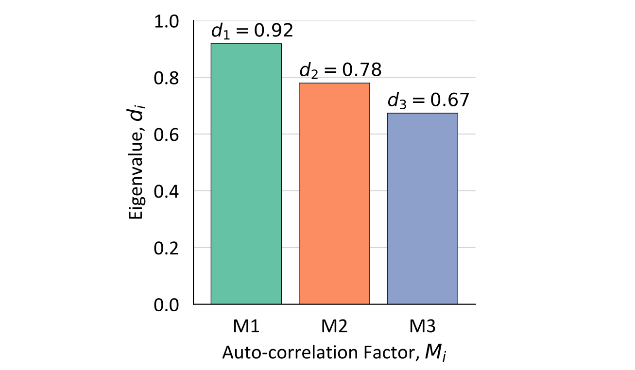
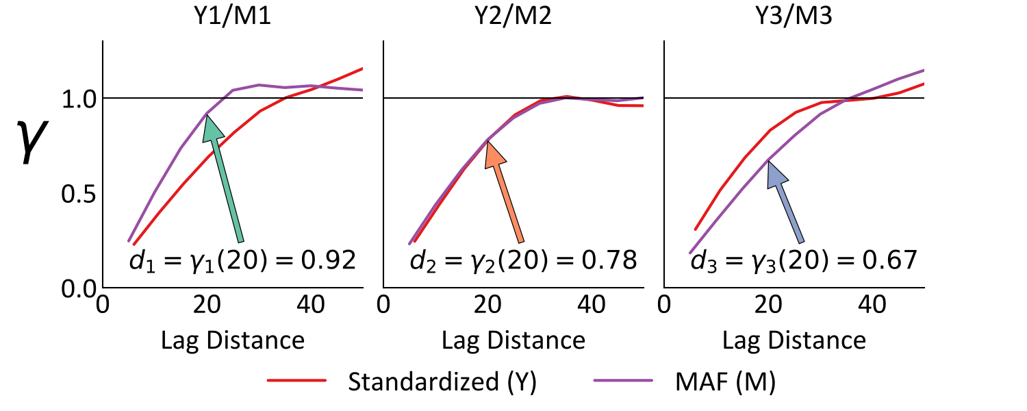
The derivation of the MAF name is therefore explained, as the factors range between the minimum and maximum autocorrelation at the chosen lag distance. Since the cross-correlation of the factors is zero at \(\mathbf{r}\), the spatial variability of the multivariate system at \(\mathbf{r}\) is entirely explained by the autocorrelations. Returning to dimension reduction, lower ranked factors of higher spatial variability may be removed for modeling purposes, as in the case of a large \(k\), they will often describe virtually random spatial structure (e.g., pure nugget effect). This may impact the selection of the decorrelation lag distance, as using an \(\mathbf{r}\) that is closer to the smallest data spacing allows for the nugget effect to be inferred from the \(\mathbf{D}_X\) entries.

Summary

Data sphereing (DRS and SDS) and MAF are extensions of PCA, providing decorrelation of the variables at \(h=0\), in addition to the following features:

1. DRS standardizes the decorrelated variables to have unit variance, which may provide practical convenience to subsequent modeling steps. The dimension reduction functionality of PCA is preserved.
2. SDS standardizes the decorrelated variables to have unit variance, while performing a second rotation to minimize mixing of the original variables. This may be useful for geostatistical modeling, as it improves the likelihood of reproducing features that are unique to each variable. The dimension reduction functionality of PCA is not preserved.
3. MAF is applied to either DRS or SDS transformed data, applying a second spectral decomposition to decorrelate the variables at one \(h>0\) lag distance. This spatial decorrelation will generally make the modeling assumption of independence more appropriate.

Readers using a web browser may find the following interactive figure useful for understanding the nature of each transform, through comparing scatter of the original variables and transformed variables. Buttons on the left may be used for toggling the displayed data, while zooming and rotation functionality is available.

Scatterplots of the original and transformed data. Use the buttons on the left to view each transform.

While these linear rotations are powerful geostatistical tools, the presence of multivariate complexities will often lead to problematic modeling results. These complexities are not captured by the covariance parameter, so that dependence will exist following decorrelation, leading to major issues with the modeling assumption of independence. This motivates multivariate Gaussian transforms, such as the projection pursuit multivariate transform that is reviewed in the companion lesson.

References