Learning Objectives

• Review checklist of minimum acceptance criteria for simulated realizations of continuous variable realizations in mining geostatistics.
• Formulate when and how to correct simulated realizations.
• Express best practice of simulation and model checking.

Introduction

Simulation is widely used to generate multiple realizations of grade variables. Grade realizations are generated within rock types or domains using a coordinate system that facilitates integration of large scale geological information. Simulation is not robust and the realizations have to be checked carefully. The performance of simulation can be impaired by (1) departures from strict stationarity including gradational changes and complex overlapping geological controls, (2) implementation decisions including the search and variogram parameters, and (3) inconsistencies between the conditioning data and the implicit multivariate distribution of the simulation approach. In practice, simulation can be applied as a black box system since knowing the internal workings of simulation would not change the need for checking of the simulated realizations. Practitioners must have thorough checking included as part of the simulation process; until a checklist of minimum acceptance criteria are met (Leuangthong, McLennan, & Deutsch, 2004), the simulated realizations should not be considered for resource or uncertainty assessment.

Checking

There are many algorithms and software for simulation. Each one could work as intended and give good results. The local site specific conditions of each domain could also lead a perfectly good algorithm/software to create realizations that have problems that need to be fixed by revising the data, modifying the domains, changing simulation parameters, or post processing the realizations. The following checking steps are recommended.

Visualization and Reproduction of Data

Visual inspection is not definitive. Large scale geological features appear small on a computer screen or in a virtual reality environment, the coloring of grades in artificial grid blocks is distracting and appreciating the variations in the 3D distribution of grades from one domain to another is difficult. Nevertheless, careful visual inspection of the realizations can reveal numerical artifacts, edge effects, high grades in known low grade areas (and vice versa), and unrealistic continuity or randomness. Experience from mined out areas and similar deposits forms the basis for visual inspection. Visual comparisons with models constructed with different software and modeling approaches may also identify potential problems.

The choice of an appropriate color scheme for visualization is important and somewhat personal. The standard color gradients in legacy software should be replaced by modern alternatives (see colorbrewer2.org as an example). Reviewers and auditors may prefer to use a consistent set of color schemes for checking different aspects of the realizations while facilitating comparison.

The pattern of variability away from the drill holes should look like the pattern of variability at the drill holes. There should be a natural variation in grades away from the data. The gridded nature of most simulated realizations means that some data may not be reproduced. There may be a data input error or some other problem. The simulated values at the data locations should be extracted and plotted against the data values; see below.

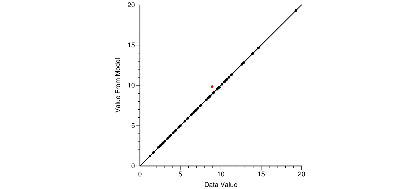
This example shows one sample (red) not reproduced by simulation because a closer one was assigned to the grid node closest to both data. The simulated value would be different for all realizations, but quite close in this case due to the low nugget effect in the variogram.

Cross Validation

Cross validation or some form of k-fold validation does not directly check the simulated realizations; however, many of the simulation parameters are tested. The standard cross validation where each drillhole is left out one at a time is practical in most cases. A more complete k-fold validation is more difficult to implement and interpretive steps like variogram modeling tend to be the same. The results should be checked in estimation mode and in probabilistic mode.

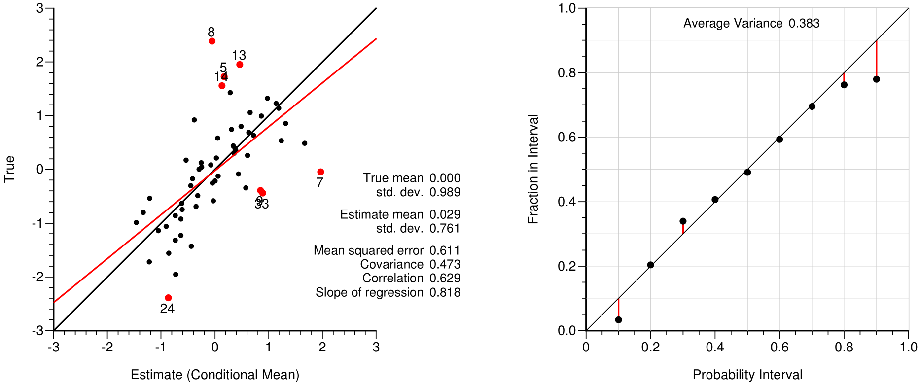
The simple kriged mean of the normal score values is the conditional mean of the local distribution and could be considered as an estimate. As shown on the left, the mean values should be similar, the mean squared error should be low, the slope of regression should be close to one, and data that are significantly over- or under-estimated (the red dots on the left plot) should be investigated. The points on the accuracy plot summarize the fairness of the predicted uncertainty. Points close to the 45 degree line indicate fair or accurate probabilities. There are less than 60 drill holes in this example and the departure from the 45 degree line is considered acceptable. The average variance is a measure of precision; the lower this average variance the more precise the distributions of uncertainty.

Reproduction of Statistical Parameters

The histogram, variogram and other statistical parameters such as the correlation coefficient to secondary data or to other simulated variables should be reasonably reproduced. The following shows the results from a small thickness variable simulation.

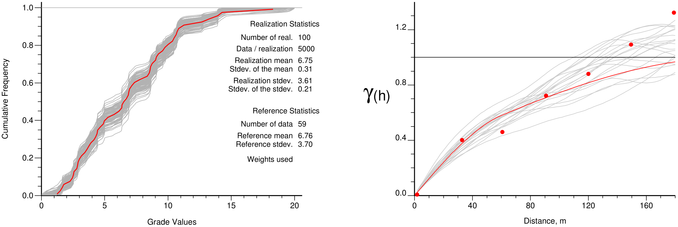
The declustering was adjusted to achieve the very close reproduction in the mean values (6.75m in the realizations and 6.76m from the declustered distribution. Note that the variograms of the simulated realizations (gray lines on the right) are closer to the experimental points than the fitted red model. This shows the expected influence of data conditioning.

Parameter uncertainty is being increasingly considered in geostatistical simulation. Each step in the process of including parameter uncertainty should be checked. The final check of the histogram and variogram could consider the base case reference results. The simulation process will update the input parameter uncertainty by conditioning to data and clipping to domain boundaries.

Swath Plots

Swath plots in principal directions are used to check reproduction of trends and the data. Each of the three principal directions are defined by an azimuth and dip. The “swaths” are perpendicular to the direction vector with some distance tolerance. The average of the data in each swath is compared to the average of the realizations. An example with 20 realizations is shown below.

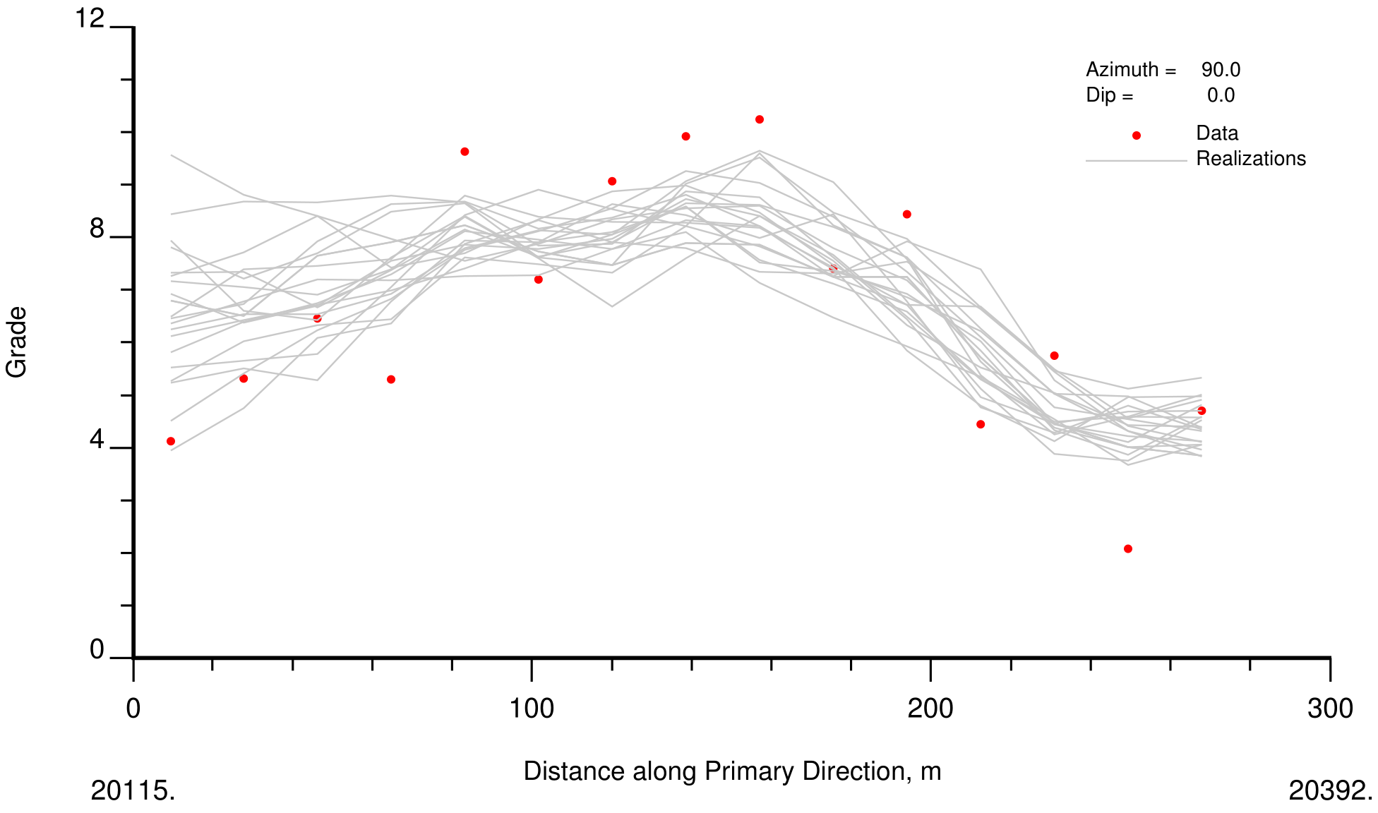
Although the realizations appear to have too high values for the first 60m, the kriging shows similar behavior and this is not considered to be a problem. Deviations may occur in sparsely sampled regions of the simulated domain. A correction to kriging could be considered if this is deemed unacceptable (see below).

Average versus Kriging

The average over multiple realizations at each location should match a kriged (or perhaps cokriged) estimate at the same location using reasonable parameters. A comparison to kriging should be performed as part of simulation checking. The plot below summarizes what should be checked: (1) a visualization of an ordinary kriged model with a reasonably large search and the average of the realizations, and (2) a cross plot between the average and the kriged model. The correlation should be larger than 0.97.

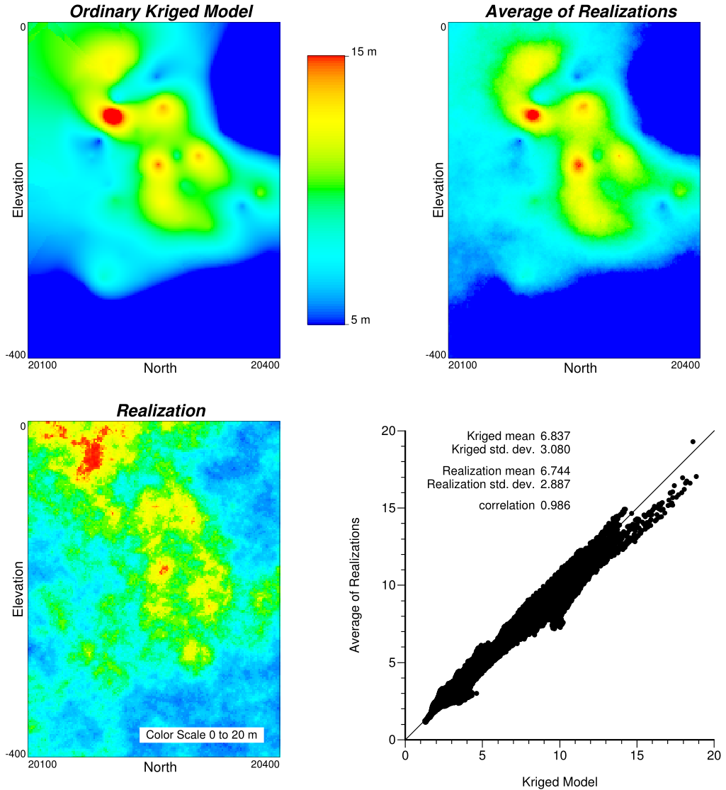
The example shown above is reasonable. The difference in the averages is about 1.5% and is marginally acceptable; a difference of less than 1% is preferred. The realizations are slightly conservative and the difference is explainable by the declustering. The declustering could be reconsidered if this difference is considered too large.

Other Checks

There are the normal checks that are performed in mining including comparison to previous or legacy models and reconciliation with production sampling and process measurements. Changing the data (ie: by the addition of new drilling information) and modeling parameters are understood by running the model with new parameters and old data, then old parameters and new data. All changes in mineral resources should be understood and the simulated realizations should provide a reasonable model of uncertainty.

Correction

Errors or mistakes should be fixed. It is possible, but not likely that modern simulation software has errors. The parameters must be carefully set. The input parameters could be wrong or entered wrong. Sometimes we have to start over with a new project and reload the data. Some other options when trying to track down problems include (1) running unconditional realizations - the data cannot interfere with the results, (2) running with a pure nugget variogram - the variogram cannot interfere with the results, (3) running the simulation for the full grid and avoiding clipping by domain boundaries - this mitigates issues due to non-stationarity and clipping.

In presence of significant issues with stationarity, that is, location dependence of the modeling parameters, soft boundaries,… the simulated realizations may be globally acceptable, but locally biased. One effective correction for simulated realizations that are not respecting the local data with enough precision is to correct all of the realizations at each location so that the average exactly matches kriging. The kriging should consider a large enough search to be conditionally unbiased and relatively free of artifacts; often ordinary kriging (OK) with 20 to 50 data is applied.

The corrected value \(\hat z\) of the random variable \(z\) for realization \(l\) at location \(\textbf{u}\) is generated using the ordinary kriged estimate \(z_{OK}\) and all \(L\) realizations at the node location. This process is repeated over the entire simulated domain \(A\).

\[ \hat z({\textbf{u}};l) = z({\textbf{u}};l) \cdot \frac{z_{OK}({\textbf{u}})}{\frac{1}{L} \sum z({\textbf{u}};l)}, \ \ l=1,...,L, \ \ {\textbf{u}} \in A \]

This correction does not substantially change the uncertainty, does not introduce negative realizations, and does not meaningfully change the local uncertainty; however, any artifacts in kriging due to a restricted search will show up in the realizations and the uncertainty will be influenced by the correction.

Another possible correction is the quantile-to-quantile correction similar to what is used in the normal score transform (like the trans approach in GSLIB (Deutsch & Journel, 1998). Considering the representative distribution \(F_{rep}\) and the distribution from the realizations (\(F_L\)), the following would correct node values to exactly match the representative distribution:

\[ \hat z_1({\textbf{u}};l) = F_{rep}^{-1} ( F_L (z({\textbf{u}};l)) ), \ \ l=1,...,L, \ \ {\textbf{u}}\in A \]

The corrected values are denoted \(\hat z_1\). The issue with this correction is that the data values can be changed. A progressive change away from the data is recommended where there is no change when the kriging variance is zero and the change is larger far away from the data:

\[ \hat z({\textbf{u}};l) = z({\textbf{u}};l)+(\hat z_1({\textbf{u}};l)-z({\textbf{u}};l) ) \cdot \frac{\sigma_{OK}^2({\textbf{u}})}{\sigma_{max}^2}, \ \ l=1,...,L, \ \ {\textbf{u}} \in A \]

The sill of the variogram (denoted as \(\sigma_{max}^2\)) is used to scale the ordinary kriging variance \(\sigma_{OK}^2\). This last correction may have to be applied multiple times (\(\hat z_i, i=1,...,N\)) to ensure histogram reproduction since the progressive change will not ensure histogram reproduction in one application. One reasonable approach is to fix the distribution of all realizations at the same time and allow each realization to fluctuate. These corrections should only be considered when there are significant problems with the original realizations, say a global difference of 3% or more in the mean grade or local changes that are clearly evident on the swath plots. The use of a correction scheme must be documented carefully, the corrected realizations must be checked again and changes to the uncertainty must be understood.

Checklist

The following should be checked:

1. Data are reproduced and realizations have no visual artifacts.

2. Cross validation of conditional mean values appears reasonable plus the distributions of uncertainty are accurate and as precise as possible.

3. Histogram and variogram are reasonably reproduced within their uncertainty.

4. Swath plots in principal directions show that the realizations reasonably match gradational trends.

5. The average of many realizations matches a kriged model constructed with a reasonable (not artificially limited) search.

6. The resources from the realizations reconcile with production data and have understandable differences from legacy models.

Summary

Simulation depends more on stationarity than the standard kriging techniques used in mining geostatistics. There are also more input parameters in simulation and more places where errors or inconsistencies can be introduced. Best practice is to have careful checking embedded in the simulation workflow; the simulation is not complete until it has been thoroughly checked.

References